R-Squared (\(R^2\)) Explained: How To Interpret The Goodness Of Fit In Regression Models

When you train a regression model, you usually want to answer a simple question:

How well does this model explain the variation in the target variable, compared with a very simple baseline?

The usual baseline is a model that always predicts the mean of the target variable. R-Squared (\(R^2\)) quantifies exactly how much better your model is compared to that simple baseline of guessing the average.

• If your model is perfect, \(R^2 = 1\) (or 100 % of variance explained).
• If your model is no better than predicting the mean, \(R^2 = 0\).
• If your model is worse than the mean, \(R^2\) becomes negative.

This article builds intuition first, then moves to the equations and implementation, and finally discusses practical tips and pitfalls.

Visualizing the Concept

Let us visualize this to make it concrete.

1. The Baseline (The Mean Model):
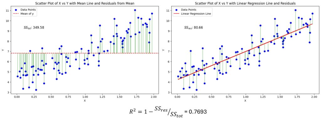
Imagine a scatter plot of house sizes vs. prices. Draw a horizontal line across the chart at the average price (\(\bar{y}\)).

• The vertical distance from each data point to this horizontal line represents the error of the baseline.
• If we square all these distances and add them up, we get the Total Sum of Squares (\(SS_{tot}\)). This represents the total variation inherent in the data.

2. Your Regression Model:
Now, draw your regression line through the data points. It should hug the points much closer than the flat horizontal line.

• The vertical distance from each data point to your regression line is the residual (the error of your model).
• If we square these residuals and sum them up, we get the Residual Sum of Squares (\(SS_{res}\)). This represents the variation that your model failed to explain.

The Intuition:
R-squared simply compares these two sums. It asks: “What fraction of the total variation (\(SS_{tot}\)) did we eliminate by using the regression line instead of the flat line?”

Math Behind R-Squared

Now that we have the intuition, let us formalize this with the mathematical definitions.

The R-squared metric is defined as:

$$ R^2 = \frac{SS_{tot} – SS_{res}}{SS_{tot}} = 1 – \frac{SS_{res}}{SS_{tot}}. $$

Where:

1. \(SS_{res}\) (Residual Sum of Squares):
   $$ SS_{res} = \sum_{i=1}^{n} (y_i – \hat{y}_i)^2 $$
   Here, \(y_i\) is the actual value and \(\hat{y}_i\) is the predicted value from your model. This term measures the error remaining after fitting the model.
2. \(SS_{tot}\) (Total Sum of Squares):
   $$ SS_{tot} = \sum_{i=1}^{n} (y_i – \bar{y})^2 $$
   Here, \(\bar{y}\) is the mean of the observed data. This term measures the total variance in the dataset.

Interpretation

• \(\frac{SS_{res}}{SS_{tot}}\): This fraction represents the percentage of variance that is unexplained by the model.
• \(1 – \dots\) : Therefore, the result represents the percentage of variance that is explained by the model.

For example, an \(R^2\) of 0.85 means that 85% of the variation in the target variable can be explained by the input features.

import numpy as np
from sklearn.linear_model import LinearRegression
from sklearn.metrics import r2_score

# 1. Generate some synthetic data
np.random.seed(42)
X = 2 * np.random.rand(100, 1)
y = 4 + 3 * X + np.random.randn(100, 1) # y = 4 + 3x + noise

# 2. Fit a Linear Regression Model
model = LinearRegression()
model.fit(X, y)
y_pred = model.predict(X)

# 3. Calculate R-squared using scikit-learn
r2_sklearn = r2_score(y, y_pred)
print(f"R-squared (sklearn): {r2_sklearn:.4f}")

# 4. Calculate R-squared Manually (The "First Principles" way)
y_mean = np.mean(y)

# Total Sum of Squares (Variance of the data)
ss_tot = np.sum((y - y_mean) ** 2)

# Residual Sum of Squares (Error of the model)
ss_res = np.sum((y - y_pred) ** 2)

# The Formula
r2_manual = 1 - (ss_res / ss_tot)
print(f"R-squared (manual):  {r2_manual:.4f}")

# Verification
assert np.isclose(r2_sklearn, r2_manual)
print("Verification successful: The manual calculation matches sklearn.")

import numpy as np
from sklearn.linear_model import LinearRegression
from sklearn.metrics import r2_score

# 1. Generate some synthetic data
np.random.seed(42)
X = 2 * np.random.rand(100, 1)
y = 4 + 3 * X + np.random.randn(100, 1) # y = 4 + 3x + noise

# 2. Fit a Linear Regression Model
model = LinearRegression()
model.fit(X, y)
y_pred = model.predict(X)

# 3. Calculate R-squared using scikit-learn
r2_sklearn = r2_score(y, y_pred)
print(f"R-squared (sklearn): {r2_sklearn:.4f}")

# 4. Calculate R-squared Manually (The "First Principles" way)
y_mean = np.mean(y)

# Total Sum of Squares (Variance of the data)
ss_tot = np.sum((y - y_mean) ** 2)

# Residual Sum of Squares (Error of the model)
ss_res = np.sum((y - y_pred) ** 2)

# The Formula
r2_manual = 1 - (ss_res / ss_tot)
print(f"R-squared (manual):  {r2_manual:.4f}")

# Verification
assert np.isclose(r2_sklearn, r2_manual)
print("Verification successful: The manual calculation matches sklearn.")

R-squared vs. RMSE

R-squared and RMSE often move together, but they answer different questions. R-squared tells you how much variance the model explains relative to a baseline, while RMSE tells you the typical size of prediction errors in the original units of the target. Looking at both side by side is essential.

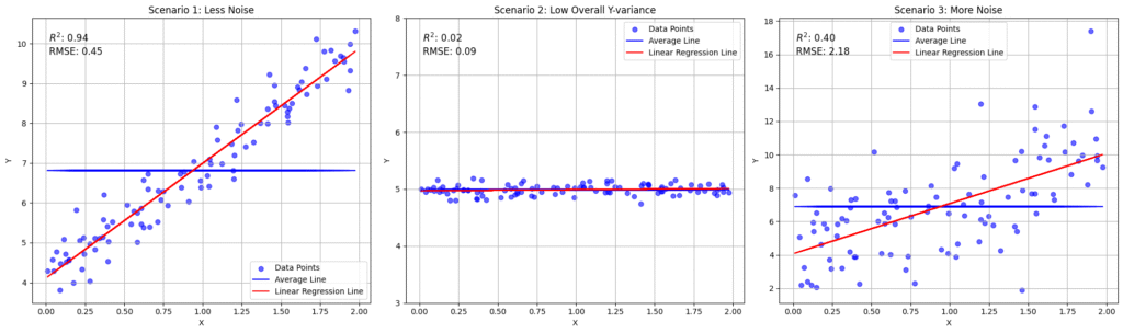
Consider three illustrative scenarios.

Scenario 1: Strong Linear Relationship with Moderate Noise

• Data: \(X\) and \(Y\) follow a clear linear trend, with points clustered reasonably tightly around the regression line.
• Metrics: \(R^2 = 0.94\), RMSE \(= 0.45\)
• Interpretation:
  The high R-squared indicates that the model explains most of the variance in the target variable. The relatively low RMSE confirms that, on average, predictions are close to the true values in absolute terms. Here, both metrics agree: the linear model is doing a very good job.

Scenario 2: Very Low Y-Variance with Poor Linear Explanation

• Data: \(X\) and \(Y\) where the target \(Y\) barely varies at all, and the feature \(X\) does not meaningfully explain what little variance exists.
• Metrics: \(R^2 = 0.02\), RMSE \(= 0.09\)
• Interpretation:
  R-squared is close to zero, indicating that the linear model explains almost none of the variation in \(Y\). However, RMSE is also very small. This is not a contradiction: RMSE is an absolute error metric. If \(Y\) itself barely moves, even a weak model can achieve low absolute error because there is simply not much variation to get wrong. In this situation, R-squared correctly signals that the model has almost no explanatory power, while RMSE looks “good” only because the underlying variance is tiny.

Scenario 3: High Noise and Weak Linear Fit

• Data: \(X\) and \(Y\) with a lot of scatter around any underlying trend, so the regression line is a poor summary of the data.
• Metrics: \(R^2 = 0.40\), RMSE \(= 2.18\)
• Interpretation:
  The relatively low R-squared indicates that the linear model captures only a modest fraction of the variance in \(Y\). The large RMSE shows that typical prediction errors are substantial in absolute terms. Together, these metrics point to either a weak linear relationship, a highly noisy process, or a mismatch between model and data.

Putting It Together

• R-squared: Measures the proportion of variance explained relative to the total variance in the target. It is a relative measure of explanatory power.
• RMSE: Measures the average magnitude of prediction errors in the same units as the target. It is an absolute measure of fit quality.

Key takeaway:
A low RMSE does not guarantee a high R-squared when the total variance of the target is very small (Scenario 2). Conversely, a high R-squared can coexist with a noticeably large RMSE if the target values live on a large numerical scale. In practice, you should interpret R-squared and RMSE together, always in the context of the problem and the scale of the data.

Practical Tips and Best Practices

While R-squared is a fundamental metric, it is often misinterpreted. Here is what you need to know to use it effectively in the real world.

1. R-squared is NOT Accuracy

A high R-squared does not necessarily mean your predictions are accurate in an absolute sense. It only means your model explains the variance well. If the variance is small to begin with, you might have a low R-squared but still have low prediction errors (RMSE). Always report R-squared alongside error metrics like RMSE (Root Mean Squared Error) or MAE (Mean Absolute Error).

2. The “Feature Creep” Problem

One major flaw of standard R-squared is that it never decreases when you add more features to the model. Even if you add a completely irrelevant feature (like “random noise”), the model will find a tiny, coincidental correlation, and R-squared will tick up slightly.

Solution: Use Adjusted R-squared.
$$ R^2_{adj} = 1 – (1-R^2) \frac{n-1}{n-p-1} $$
Where \(n\) is the number of samples and \(p\) is the number of predictors. Adjusted R-squared penalizes the model for adding useless features. If a new feature genuinely improves the model, adjusted \(R^2\) will increase. If the feature only adds noise, adjusted \(R^2\) will often decrease.

3. R-squared Can Be Negative

This surprises many beginners. If \(R^2 < 0\), it means your model is worse than the baseline. $$ SS_{res} > SS_{tot} $$
This implies that your model’s predictions are further away from the actual values than the simple mean of the data. Situations where this can occur include:

• You fit a model without an intercept (for example, forcing the regression line through the origin).
• You evaluate the model on a different dataset from the one it was trained on (for example, a test set with a different distribution), and performance is poor.
• You use a model that is structurally inappropriate for the problem (for example, fitting a linear model to a strongly nonlinear relationship without suitable features).

In practice, a negative \(R^2\) should trigger a careful check of the modeling assumptions and data preprocessing steps.

4. What Counts as a “Good” R-Squared?

There is no universal threshold for a “good” \(R^2\). The interpretation is domain dependent.

• In controlled physical or engineering systems, an R-squared of 0.95 might be considered low.
• In social sciences, marketing, or behavioral prediction, an R-squared of 0.30 might be considered a breakthrough.

Instead of relying on mental thresholds, you should:

• Compare your model against simple baselines (for example, the mean model or a univariate regression).
• Compare against established benchmarks in your domain.
• Look at error distributions and residual plots, not just a single scalar.

5. Limitations: When Not to Rely on R-Squared

R-squared can be misleading in several situations:

• Nonlinear models: For complex models (for example, tree ensembles, neural networks), \(R^2\) is still defined but does not provide insight into the functional form or stability of the model.
• Heteroscedasticity: If the variance of the errors changes with the predicted value, \(R^2\) alone hides this issue; residual plots are more informative.
• Outliers: A few extreme points can inflate or deflate \(R^2\) dramatically.
• Time series: In time-dependent data, naive baselines like “use the last value” can outperform the mean, making plain \(R^2\) less relevant. Specialized metrics or baselines are more appropriate.

The general message is: treat \(R^2\) as one piece of evidence, not the sole criterion for model quality.

Summary

R-squared provides a simple, normalized measure of how much of the original variance in the target variable is captured by a regression model, relative to a mean-only baseline.
It is the bridge between “how much variation exists” and “how much variation we understand.” By comparing our model’s errors against the natural variance of the data, it gives us a normalized score of explanatory power.

Use it to understand the strength of the relationship, but rely on error metrics (RMSE) to understand the precision of the predictions.