Imagine you’re trying to teach a world-class chef a new recipe. Instead of retraining them from scratch, you just show them a few tweaks—maybe a new spice or a different cooking technique. They adapt quickly, leveraging their vast experience while only changing what’s necessary. This is the essence of Parameter Efficient Fine-Tuning (PEFT) in machine learning: adapting large, pre-trained models to new tasks by updating only a small subset of their parameters.
Why PEFT?
Large language models (LLMs) and vision models are like expert chefs—they’ve learned a lot from massive datasets. But when you want them to master a new dish (task), retraining the whole model is expensive and often unnecessary. PEFT methods let us fine-tune just a few ingredients (parameters), making adaptation faster, cheaper, and more accessible.
What is PEFT? (Conceptual Overview)
Parameter Efficient Fine-Tuning refers to a family of techniques that adapt pre-trained models to new tasks by updating only a small fraction of their parameters. The rest of the model remains frozen, preserving the knowledge learned during pre-training.
Why is this important?
- Resource Efficiency: Fine-tuning billions of parameters is costly in terms of compute, memory, and storage. By drastically reducing the need for high-end GPUs, PEFT allows more people to experiment with and build on state-of-the-art models.
- Faster Training: With fewer parameters to update, training is much quicker.
- Better Generalization: By not overfitting the entire model, PEFT can help retain the general knowledge from pre-training.
- Reduces Catastrophic Forgetting: When you fine-tune all parameters of a model, it can “forget” some of the general knowledge it learned during pre-training. By keeping most weights frozen, PEFT helps prevent this.
- Enables Multi-Task Learning: You can train several lightweight PEFT modules for different tasks and swap them out as needed, all while using the same base model. This is incredibly efficient.
How Does PEFT Work? (Technical Deep Dive)
Let’s break down the most popular PEFT methods:
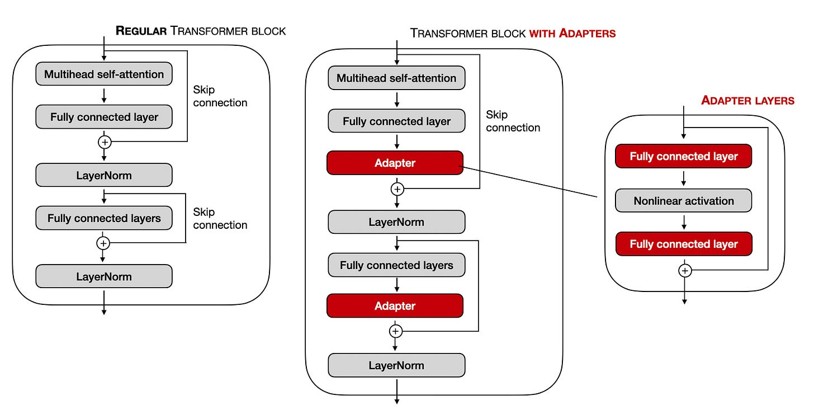
1. Adapter Layers
Adapters are small, specialized neural network modules inserted between the existing layers of a pre-trained model. During fine-tuning, we only train the adapters, leaving the massive original model untouched.
Imagine a skyscraper representing our pre-trained model. Each floor is a layer. To adapt the building for a new purpose, we don’t tear down walls. Instead, we install a small, pre-fabricated “adapter pod” on each floor. These pods contain a new function—like a mini-office or a coffee station. The building’s core structure remains the same, but its capabilities are now extended.
The adapter is a bottleneck: it first projects the high-dimensional input to a smaller dimension, processes it, and then projects it back up, ensuring it’s lightweight.
If \(h\) is the output of a transformer layer (our hidden state), the adapter modifies it like this:
\[
h’ = h + f_{adapter}(h)
\]
where \(f_{adapter}\) is the small bottleneck MLP. This addition is a residual connection, allowing the model to learn the identity function if the adapter isn’t needed.
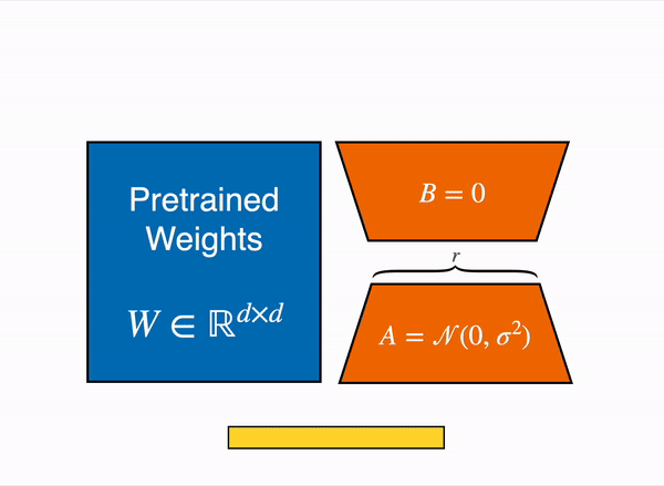
2. LoRA (Low-Rank Adaptation)
LoRA is a clever technique that avoids touching the original weights at all. It injects trainable low-rank matrices into the attention or feed-forward layers.
Imagine a wide river (the weight matrix). Instead of redirecting the whole river, you build a small canal (low-rank update) that influences its flow.
Instead of updating the full weight matrix $W$, we approximate the change $\Delta W$ with a low-rank decomposition:
$$
W’ = W + \Delta W = W + BA
$$
Here, \(W \in \mathbb{R}^{d \times k}\) is the original, frozen weight matrix. The update is composed of two much smaller matrices, \(B \in \mathbb{R}^{d \times r}\) and \(A \in \mathbb{R}^{r \times k}\), where the rank \(r\) is tiny compared to \(d\) and \(k\). We only train the parameters of \(A\) and \(B\).
3. Prompt Tuning / Prefix Tuning
These methods take a different approach: they don’t change the model’s weights at all. Instead, they introduce a small, trainable “prompt” or “prefix”—a vector of parameters—that is fed into the model alongside the actual input. The model learns to interpret this prefix as a command to perform a specific task.
Think of giving the model a cheat sheet at the start of every exam. The core knowledge is unchanged, but the cheat sheet guides its answers for the new task.
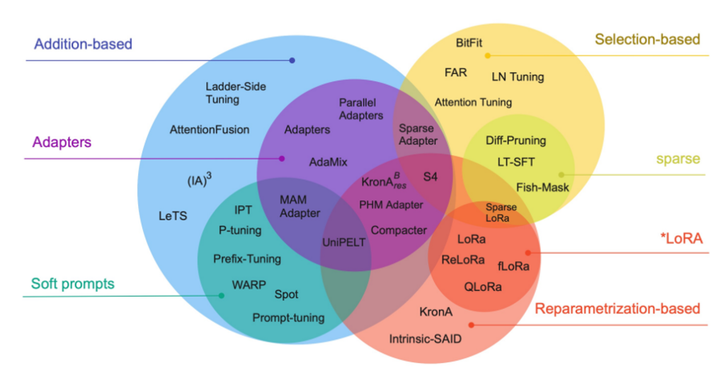
4. Other PEFT Methods and Categories
The methods we’ve discussed—Adapters, LoRA, and Prompt Tuning—are the most popular, but they belong to a broader family of techniques. A helpful way to categorize PEFT methods is based on how they modify the model during fine-tuning [Lialin et al.]:
- Additive Methods: These introduce new, trainable parameters while keeping the original model weights frozen. This is like adding a new wing to a building without altering the original structure.
- Examples: Adapters and Prompt/Prefix Tuning fall into this category.
- Selective Methods: These fine-tune only a small subset of the existing model parameters. This is the simplest approach, where you might only update the bias terms or the final few layers of the network.
- Example: Fine-tuning only the bias parameters (
BitFit) or the top two layers of a transformer.
- Example: Fine-tuning only the bias parameters (
- Reparameterization-based Methods: These reparameterize the model’s weights using a low-rank or compressed representation. Only the parameters of this new, efficient representation are trained.
- Example: LoRA is the prime example, representing the weight update as a low-rank product of two smaller matrices.
Practical Example: LoRA with PyTorch
Let’s see how LoRA can be implemented in practice. Here’s a simplified PyTorch example:
import torch
import torch.nn as nn

class LoRALinear(nn.Module):
    def __init__(self, in_features, out_features, r=4):
        super().__init__()
        # The original, frozen linear layer
        self.linear = nn.Linear(in_features, out_features)
        # LoRA parameters
        self.A = nn.Parameter(torch.randn(r, in_features) * 0.01)
        self.B = nn.Parameter(torch.randn(out_features, r) * 0.01)
        # Freeze original weights
        self.linear.weight.requires_grad = False
        self.linear.bias.requires_grad = False

    def forward(self, x):
        # The original, pre-trained path
        original_output = self.linear(x)
        # The low-rank update path
        lora_update = (self.B @ self.A) @ x.T
        # Combine the two paths
        return original_output + lora_update.T

# Example usage: Let's assume a model with hidden size 768 and we choose a rank of 8
layer = LoRALinear(768, 768, r=8)
input = torch.randn(32, 768) # A batch of 32 inputs
output = layer(input)
# During training, only self.A and self.B will have their gradients computed!Real-World Applications
- Chatbots and Virtual Assistants: Quickly adapt LLMs to specific domains (e.g., medical, legal) without retraining the whole model.
- Edge Devices: Deploy large models on resource-constrained hardware by only storing and updating small adapter weights.
- Rapid Prototyping: Experiment with new tasks or datasets with minimal compute.
Summary Table: PEFT Methods at a Glance
| Method | What’s Tuned? | Storage Overhead | Typical Use Case |
|---|---|---|---|
| Adapters | Small MLPs per layer | Low | Multi-task, domain adapts |
| LoRA | Low-rank matrices | Very Low | LLMs, transformers |
| Prompt Tuning | Input embeddings | Very Low | NLP, few-shot learning |
Final Thoughts
Parameter Efficient Fine-Tuning is revolutionizing how we adapt large models. By focusing on intuition, visual analogies, and practical code, we can make these powerful techniques accessible to everyone—from researchers to engineers. The next time you want to teach your model a new trick, remember: sometimes, a sticky note is all you need.

Silpa brings 5 years of experience in working on diverse ML projects, specializing in designing end-to-end ML systems tailored for real-time applications. Her background in statistics (Bachelor of Technology) provides a strong foundation for her work in the field. Silpa is also the driving force behind the development of the content you find on this site.
Subscribe to our newsletter!