Weight initialization in neural networks significantly influences the efficiency and performance of training algorithms. Proper initialization strategies can prevent issues like vanishing or exploding gradients, accelerate convergence, and improve the generalization capabilities of models.
Why Weight Initialization Matters
In the training of neural networks, especially deep networks, weight initialization can have profound impacts on the training dynamics. Consider the following consequences of poor weight initialization:
- Vanishing Gradients: When weights are initialized too close to zero, the gradients during backpropagation can become exceedingly small, hindering learning.
- Exploding Gradients: Conversely, overly large weights can lead to excessively large gradients, causing instability in the weight updates.
- Symmetry Breaking: If all weights are initialized to the same value (e.g., zeros), the neurons will learn the same features during training—thus failing to exploit the representational powers of multiple neurons.
- Convergence Speed: Proper initialization can lead to faster convergence when training, reducing the time taken to reach optimal or near-optimal solutions. Poor initialization can lead to slow convergence or getting stuck in local minima.
Typical Weight Initialization Challenges
- Distance from optimal values: Initializing weights too far from their optimal values can prolong convergence.
- Gradient Flow: Properly maintaining gradient flow across layers is essential for deep networks.
- Biases: While weights dictate the behavior of connections between neurons, biases also need thoughtful initialization to ensure that neurons activate appropriately.
Common Weight Initialization Techniques
Over the years, various weight initialization techniques have been developed, with each catering to specific architectures and non-linear activation functions. Below, we explore the most common techniques in detail.
1. Random Initialization
Concept: Weights are initialized randomly, often from a Gaussian distribution or uniform distribution with a mean close to zero.
Formulation:
- Gaussian: \(W \sim \mathcal{N}(0, \sigma^2)\)
- Uniform: \(W \sim \mathcal{U}(-\epsilon, \epsilon)\) where \(\epsilon\) is a small positive value.
Pros: Breaks symmetry, providing each neuron with distinct gradients.
Cons: If the range is too small (close to zero), it can lead to vanishing gradients. If too large, it can cause exploding gradients.
2. Xavier/Glorot Initialization
Concept: The Xavier initialization method, named after Xavier Glorot, is particularly suited for sigmoid and hyperbolic tangent activation functions.
Formulation:
\[
W \sim \mathcal{U}\left(-\frac{\sqrt{6}}{\sqrt{n_{in}+n_{out}}}, \frac{\sqrt{6}}{\sqrt{n_{in}+n_{out}}}\right)
\]
where \(n_{in}\) and \(n_{out}\) are the number of incoming and outgoing connections, respectively.
In practice, ML Engineers often initialize the Xavier weights from a normal distribution:
\[
W \sim \mathcal{N}(0, \frac{2}{n_{in} + n_{out}})
\]
Pros: Maintains the variance of activations across layers, thereby aiding in effective gradient flow. Best suited for activation functions like sigmoid or hyperbolic tangent (tanh).
Cons: Might not be optimal for ReLU activation functions.
3. He Initialization
Concept: He initialization [paper], designed for ReLU and its variants, addresses the shortcomings of Xavier initialization when using functions like ReLU, which can zero out negative inputs.
Formulation:
\[
W \sim \mathcal{N}\left(0, \frac{2}{n_{in}}\right)
\]
or for uniform distribution:
\[
W \sim \mathcal{U}\left(-\sqrt{\frac{6}{n_{in}}}, \sqrt{\frac{6}{n_{in}}}\right)
\]
Pros: Prevents dying neurons (inactive ReLU distributions) and maintains variance effectively. By scaling only with the number of input neurons, He initialization accounts for the ReLU’s behavior, which tends to output zeros for negative inputs.
4. LeCun Initialization
Concept: Specifically tailored for activation functions like sigmoid, Leaky ReLU, SELU, and tanh, this initialization method also seeks to maintain the variance across layers.
Formulation:
\[
W \sim \mathcal{N}\left(0, \frac{1}{n_{in}}\right)
\]
or for uniform distribution:
\[
W \sim \mathcal{U}\left(-\sqrt{\frac{3}{n_{in}}}, \sqrt{\frac{3}{n_{in}}}\right)
\]
Pros: Works well for models employing Leaky ReLU and other functions, preserving gradient flow even in deeper architectures. By using the reciprocal of the number of input neurons, it helps in maintaining the gradient’s scale throughout the layer transitions, controlling the flow of information during training.
5. Orthogonal Initialization
Concept: Orthogonal initialization generates weight matrices that are orthogonal, meaning that their rows and columns are perpendicular vectors. This preserves the inner product dynamics of activations throughout layers.
Formulation: If \(W\) is a weight matrix, find \(W\) such that \(W^T W = I\).
Pros: Empirically shown to improve convergence speed and robustness, particularly in recurrent neural networks.
6. Factorized Initialization
This method involves splitting weight matrices into lower-dimensional factors to help mitigate the vanishing and exploding gradient problems.
Intuition: Inspired by techniques such as matrix factorization, factorized initialization considers the underlying structure and ensures better control over the gradients.
Applications: Useful in specific NLP settings, particularly in sequence models.
7. Custom Initialization Strategies
In some cases, researchers and practitioners may develop custom initialization strategies based on empirical observations or specific requirements of a model:
Task-Specific Initialization: Leveraging prior knowledge or insights about the problem being solved can inform a strategy that optimally initializes the weights.
Pre-trained Weights: Utilizing weights trained from a related task (transfer learning) can accelerate the convergence process, particularly in scenarios where data is limited.
Best Practices in Weight Initialization
- Use Specific Initializations for Activation Functions: Choose initialization strategies that align with the non-linearities used in your networks (e.g., He for ReLU, Xavier for tanh).
- Keep it Random: Avoid deterministic weight initialization; incorporate randomness to break symmetry and improve exploratory behavior during training.
- Monitor Gradient Flow: Use training diagnostics (loss curves, gradient norms) to assess the efficacy of your weight initialization strategy.
- Experiment and Iterate: Conduct systematic experiments with various weight initializations alongside regularization techniques to find an optimal combination that can enhance model performance.
Metrics for Evaluation of Weight Initialization Techniques
When evaluating the goodness of a weight initialization method, the following metrics can be critical:
- Convergence Rate: The number of epochs or iterations required to reach a certain loss threshold.
- Final Loss/Accuracy: Performance on validation or test sets as a proxy for generalization.
- Gradient Distribution: Monitoring gradients to visualize any issues related to vanishing or exploding gradients.
Summary
- Starting all weights equally (zero or constant) causes them to update identically during training. They all behave similarly, hindering the network’s ability to learn effectively. This is known as the symmetry-breaking problem.
- If the initial weights are very small, the signals flowing through the network gradually weaken as they pass through multiple layers. This leads to extremely small gradients, making it difficult for the network to learn. Conversely, if the initial weights are too large, the neuron activations become “saturated” (their output stops changing significantly), also resulting in vanishing gradients during the learning process.
- To ensure stable and effective training, the initial weights should be drawn from a distribution with an appropriate variance. If the variance is too small or too large, it can lead to problems during training. A variance of approximately 1 is generally considered a good starting point.
- Xavier or Glorot initialization is a well-established method for networks that use activation functions like sigmoid and tanh. These functions have a mean output of zero, making this initialization technique suitable.
- ReLU is a popular activation function, but it doesn’t have a mean output of zero. In such cases, He initialization is generally recommended as it is specifically designed to work well with ReLU and similar activation functions.
References
Silpa brings 5 years of experience in working on diverse ML projects, specializing in designing end-to-end ML systems tailored for real-time applications. Her background in statistics (Bachelor of Technology) provides a strong foundation for her work in the field. Silpa is also the driving force behind the development of the content you find on this site.
Subscribe to our newsletter!


