Low-Rank Adaptation (LoRA) is a novel and efficient method for fine-tuning large language models (LLMs). By leveraging low-rank matrix decomposition, LoRA allows for effective adaptation of pre-trained models to specific tasks with significantly fewer trainable parameters.
What is LoRa?
LoRa is a technique that introduces low-rank matrices into the architecture of pre-trained models. Instead of updating all the parameters of the model during fine-tuning, LoRa reduces the number of trainable parameters by using low-rank decomposition. This allows for efficient adaptation with minimal impact on the original model weights.
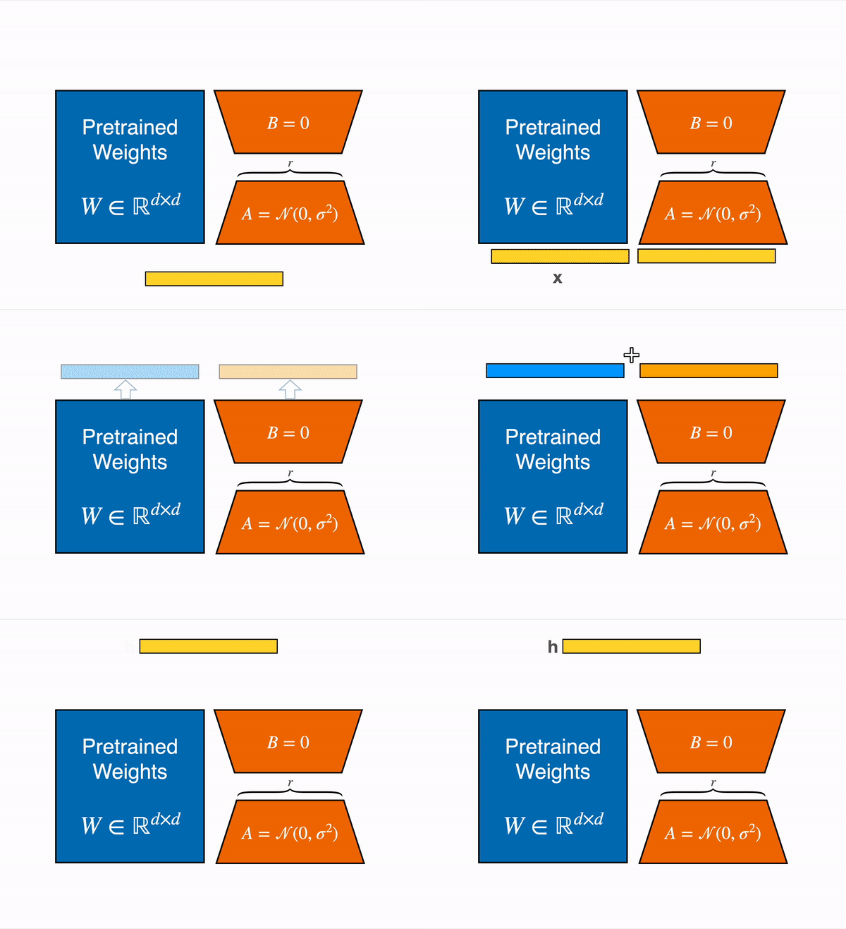
LoRA Vizualization (Source)
Theoretical Foundations
- Objective: Fine-tune pre-trained LLMs while minimizing resource usage.
- Key Idea: Instead of updating all parameters, LoRA introduces low-rank matrices into the model architecture, allowing for parameter-efficient tuning.
Weight Decomposition: (Compressed Parameter Representation)
For a weight matrix \( W \) of size \( m \times n \): \[ W \approx W_0 + \Delta W \] \( W_0 \): The original pretrained weights. \( \Delta W \): The update weights to be learned, expressed as the product of two low-rank matrices: \[ \Delta W = A B \] where:
- \( A \) is of size \( m \times r \)
- \( B \) is of size \( r \times n \)
- \( r \) is the rank (much smaller than \( m \) and \( n \))
Parameterization: (LoRA Configuration)
- A small number of parameters are introduced via the low-rank matrices \( A \) and \( B \):
\[ \text{Number of parameters} = m \cdot r + r \cdot n \] - The efficiency arises from \( r \ll m \) and \( r \ll n \).
Forward Pass Adjustment:
- Given a layer in the model, where \( x \) is the input:
\[ \text{Output} = W \cdot x \approx (W_0 + A B) \cdot x \] - This allows the forward pass to incorporate the low-rank update without modifying the original weights significantly.
Loss Calculation: (Training Objective)
- The training objective remains to minimize a loss function \( \mathcal{L} \):
\[ \mathcal{L} = \sum (\text{True Labels} – \text{Predicted Outputs})^2 \] - The gradients with respect to the low-rank updates \( (A, B) \) must then be calculated:
\[ \frac{\partial \mathcal{L}}{\partial A}, \quad \frac{\partial \mathcal{L}}{\partial B} \]
Step-by-Step Fine-Tuning Process with LoRA
Step 1: Initial Setup
- Select a Pre-trained Model: Choose a suitable pre-trained language model (e.g., BERT, GPT).
- Define Hyperparameters: Set the rank \( r \) for the low-rank matrices, learning rate, batch size, etc.
Step 2: Introduce Low-Rank Matrices
- Initialize Matrices:
- Create matrices \( A \) and \( B \) initialized with small random values or zeros.
Step 3: Modify Model Architecture
- Layer Modification: For each weight matrix \( W \) that you want to adapt:
- Introduce \( A \) and \( B \) such that:
\[ \text{New Weight} = W_0 + A B \]
Step 4: Prepare for Training
- Freeze Original Weights: Keep \( W_0 \) static to retain knowledge during the fine-tuning process.
Step 5: Training Loop
- Forward Pass: For each input \( x \):
- Compute the model output using the modified weights.
- Compute Loss: Calculate the training loss, \( \mathcal{L} \).
- Backpropagation: Compute gradients:
- Use the chain rule to find:
\[ \frac{\partial \mathcal{L}}{\partial A}, \quad \frac{\partial \mathcal{L}}{\partial B} \]
Step 6: Update Parameters
- Gradient Descent: Update \( A \) and \( B \) using an optimization algorithm (e.g., Adam):
\[ A \leftarrow A – \eta \frac{\partial \mathcal{L}}{\partial A} \]
\[ B \leftarrow B – \eta \frac{\partial \mathcal{L}}{\partial B} \]
Step 7: Evaluation
- Model Evaluation: After a sufficient number of epochs, evaluate the fine-tuned model on validation/test sets to ensure that performance is improved.
Fine-tuning LLMs with LoRa: A Step-by-Step Coding Guide
Before diving into the fine-tuning process, ensure you have the following:
- A pre-trained LLM (e.g., GPT, BERT)
- Access to a suitable dataset for the specific task
- An appropriate machine learning framework (e.g., PyTorch, TensorFlow)
- The LoRa library or implementation compatible with the chosen framework
Step 1: Setup Your Environment
- Install Required Libraries: Ensure that your environment has necessary libraries like PyTorch, Hugging Face Transformers, etc.
pip install torch transformers- Import Necessary Modules:
  import torch
from transformers import YourModel, YourTokenizerStep 2: Load the Pre-trained Model
- Load Your LLM: Use a pre-trained model from the Hugging Face hub or any other source.
  model = YourModel.from_pretrained('model_name')
tokenizer = YourTokenizer.from_pretrained('model_name')Step 3: Prepare Your Dataset
- Dataset Preprocessing: Format your dataset to be compatible with the model and tokenizer.
  from datasets import load_dataset

dataset = load_dataset('your_dataset_name')- Tokenize Your Data:
  def tokenize_function(examples):
      return tokenizer(examples['text'], padding='max_length', truncation=True, max_length=512)

tokenized_dataset = dataset.map(tokenize_function, batched=True)Step 4: Set Up LoRa
- Initialize LoRa: Implement low-rank matrices within the model architecture. This usually requires modifications to the model’s layers.
# Example: Adding LoRa layers to the model (pseudocode)
model.lora_layers = LoRALayer(input_dim, output_dim, rank)Step 5: Configure Training Parameters
- Define Training Arguments:
  from transformers import TrainingArguments

  training_args = TrainingArguments(
      output_dir='./results',
      per_device_train_batch_size=8,
      per_device_eval_batch_size=8,
      num_train_epochs=3,
      logging_dir='./logs',
      logging_steps=10,
)Step 6: Set Up the Trainer
- Initialize the Trainer:
  from transformers import Trainer

  trainer = Trainer(
      model=model,
      args=training_args,
      train_dataset=tokenized_dataset['train'],
      eval_dataset=tokenized_dataset['test'],
)Step 7: Fine-Tune the Model
trainer.train()Step 8: Evaluate the Model
trainer.evaluate()Step 9: Save the Fine-Tuned Model
  model.save_pretrained('./fine_tuned_model')
tokenizer.save_pretrained('./fine_tuned_model')Step 10: Test the Fine-Tuned Model
- Inference: Load your fine-tuned model and test its performance on new data.
  model = YourModel.from_pretrained('./fine_tuned_model')
  tokenizer = YourTokenizer.from_pretrained('./fine_tuned_model')

  inputs = tokenizer("Your test input text", return_tensors='pt')
outputs = model(**inputs)Advantages of LoRA
1. Computational Efficiency
- Reduced Resource Requirements: Since only a small subset of parameters is updated, LoRA requires significantly less computational power compared to traditional fine-tuning methods.
- Faster Training Times: Lower memory usage and fewer calculations lead to quicker training iterations.
2. Parameter Efficiency
- Less Overhead: LoRA’s low-rank matrices lead to a minimal increase in the overall model size, making it suitable for deployment in resource-constrained environments.
- Flexible Deployment: Users can easily rotate or swap tasks without needing to store multiple large models.
3. Preservation of Pre-trained Knowledge
- Retained Capabilities: By freezing the original model weights, LoRA ensures that the pre-trained knowledge of the model is preserved, reducing the risk of catastrophic forgetting.
- Better Generalization: This approach generally leads to better performance on unseen tasks as the foundational knowledge remains intact.
4. Ease of Implementation
- Straightforward Adaptation: LoRA can be integrated into existing architectures with relative ease, making it accessible for both researchers and practitioners.
- Compatibility: It is applicable across various transformer architectures and can support numerous downstream tasks.
Disadvantages of LoRA
1. Limited Expressiveness
- Rank Constraint: The low-rank assumption may limit the model’s ability to capture complex relationships in the data, especially if the rank doesn’t align well with the required capacity for certain tasks.
- Potential Performance Trade-off: For highly complex or nuanced tasks, LoRA might not achieve the same performance as full fine-tuning.
2. Task-Specific Fine-tuning
- Dependency on Task Settings: The effectiveness of LoRA can vary widely depending on the dataset and the specific task being addressed. It may require iterative experimentation to find the optimal configuration.
3. Additional Complexity
- Implementation Nuances: Although easier than full fine-tuning, LoRA introduces its own complexities in terms of managing low-rank matrices, which might not be trivial for all users.
- Need for Rank Selection: Selecting the appropriate rank hyperparameter can be non-trivial and may require expert tuning or additional experimentation time.
4. Hyperparameter Sensitivity
- Influence on Training Dynamics: LoRA often involves numerous hyperparameters that need careful tuning, impacting both training stability and final model performance.
Silpa brings 5 years of experience in working on diverse ML projects, specializing in designing end-to-end ML systems tailored for real-time applications. Her background in statistics (Bachelor of Technology) provides a strong foundation for her work in the field. Silpa is also the driving force behind the development of the content you find on this site.
Subscribe to our newsletter!


