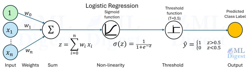
Logistic regression is a probabilistic linear classifier. It starts with a linear score, converts that score into a probability for the positive class, and then uses that probability to make a decision. That makes it one of the simplest models that gives you all three of the following at once:
- a linear decision boundary,
- an estimated probability,
- and coefficients you can often interpret directly.
At a high level:
- First, a feature vector $x$ produces a score $z = \theta^\top x$.
- Then the sigmoid turns that score into a probability:
$$p(x)=P(y=1\mid x)=\sigma(\theta^\top x), \qquad \sigma(z)=\frac{1}{1+e^{-z}}.$$
For a threshold of $0.5$, the model predicts the positive class when $\theta^\top x \ge 0$, so the decision boundary is linear even though the predicted probability is nonlinear.
Statistically, logistic regression is a Bernoulli generalized linear model (GLM) with a logit link. Practically, it is a strong first model for tabular data, risk scoring, and any classification problem where you care about fast training, stable optimization, and probabilities you can reason about.
Why it Matters
- Interpretability: Unlike a neural network black box, you can read the coefficients directly. If the coefficient for “Income” is positive, higher income increases the probability of the positive class.
- Calibrated Probabilities: It doesn’t just give you a “Yes/No”. It gives you a confidence score (e.g., “70% chance of rain”). This is crucial for risk estimation (fraud, churn, medical triage).
- Well-behaved optimization: The negative log-likelihood for logistic regression is convex in the parameters, so training is typically stable and predictable.
- Strong baseline: On many structured or tabular datasets, logistic regression is hard to beat with simple features and sensible regularization.
Core Idea: Linear Model in Log-Odds Space
The familiar sigmoid curve is not an arbitrary choice. Logistic regression assumes that the log-odds of the positive class are a linear function of the features. In other words, the model is linear in the quantity that matters for binary decisions, even though the final probability is curved.
The Geometry of Odds
The probability $p$ is bounded between 0 and 1, which makes it awkward to model directly with a linear function. The odds ratio
$$\frac{p}{1-p}$$
maps probabilities from $[0,1]$ to $[0,\infty)$, and taking the log maps them to the full real line. Logistic regression then assumes that the log-odds are linear:
$$ \log\left(\frac{p(x)}{1-p(x)}\right) = \theta^\top x $$
This equation is what makes the coefficients interpretable:
- A one-unit increase in feature $x_j$ changes the log-odds of the positive class by $\theta_j$, holding other features fixed.
- Equivalently, it multiplies the odds by a factor of $e^{\theta_j}$.
- The intercept shifts the baseline log-odds before any feature contribution is added.
One subtle but important point: a positive coefficient does not add a fixed amount to the probability itself. The effect on probability depends on the current operating point. Moving from $0.50$ to $0.60$ is much easier than moving from $0.95$ to $0.99$ because the sigmoid saturates near the extremes.
That distinction matters in practice. People often say “a feature increases the probability by X,” but logistic regression coefficients do not work that way. They act linearly on the log-odds, and only indirectly on the probability.
Training Objective: Maximum Likelihood, Not Squared Error
In linear regression, we minimize mean squared error. For logistic regression, pairing a sigmoid output with squared error leads to a poorly behaved optimization landscape in parameter space.
Instead, we use the Log Loss (or Binary Cross-Entropy), which corresponds to Maximum Likelihood Estimation:
$$ J(\theta) = -\frac{1}{m} \sum_{i=1}^{m}\Big[y^{(i)} \log(p^{(i)}) + \big(1-y^{(i)}\big)\log\big(1-p^{(i)}\big)\Big] $$
- If the true label is $1$ ($y=1$), we want $\log(p)$ to be close to 0 (so $p$ is close to 1). If $p$ is small, the penalty explodes to infinity.
- If the true label is $0$ ($y=0$), we want $\log(1-p)$ to be close to 0.
For standard logistic regression, this objective is convex in $\theta$. That does not mean every optimizer converges instantly, but it does mean training is not fighting spurious local minima the way many nonlinear models do.
Practical Optimization Notes
The gradient of this cost function is elegantly simple:
$$\nabla J(\theta) = \frac{1}{m}\sum_{i=1}^m \big(p^{(i)} – y^{(i)}\big) x^{(i)}.$$
It looks very similar to the gradient for linear regression. The only difference is that the prediction is now the sigmoid probability $p^{(i)}$ rather than a raw linear output. This gradient says: “Move the weights in the direction of the error, scaled by the input feature.”
For second-order optimization such as Newton’s method, the Hessian depends on $p(1-p)$. This term is largest at $p=0.5$ and small near 0 and 1. This means the model learns most effectively from “uncertain” examples near the decision boundary, and barely changes in response to examples it is already confident about.
Another useful interpretation is that cross-entropy punishes confident wrong predictions much more strongly than uncertain ones. Predicting $0.99$ for an example whose true label is $0$ is far worse than predicting $0.60$, and the loss reflects that sharply.
Practical Considerations for the Engineer
1. Regularization is not optional
In high dimensions, it is easy for the model to perfectly separate the training data. If a dataset is perfectly separable, the optimal weights $\theta$ are infinite (to push the sigmoid to exactly 0 and 1).
Standard practice is to add an $\ell_2$ (Ridge) or $\ell_1$ (Lasso) penalty to the cost function.
- Ridge: Keeps weights small, preventing overfitting.
- Lasso: Can zero out weights completely, performing feature selection.
In most production settings, “plain” unregularized logistic regression is the exception rather than the rule. The regularized model is usually the one you actually want.
2. The Threshold Dilemma
The model outputs a probability, say $0.65$. Is that a “Yes” or a “No”?
The default threshold is $0.5$, effectively defined by the plane $\theta^\top x = 0$.
In practice, that threshold should reflect business cost, class imbalance, and the metric you care about.
- Cancer screening: Missing a positive case (False Negative) is disastrous. You might lower the threshold to $0.1$.
- Spam filter: Deleting a real email (False Positive) is annoying. You might raise the threshold to $0.9$.
This is why model quality and decision policy are not the same thing. Logistic regression gives you a score; your product or business constraints decide how to act on that score.
3. Feature Scaling
While feature scaling is not required for the model to be valid, it is often important in practice, especially with regularization and iterative solvers.
Common choices are standardization (zero mean, unit variance) or min-max scaling. Scaling helps with:
- Convergence Speed: Gradient descent struggles with “narrow valleys” caused by unscaled features.
- Regularization Fairness: If “Income” is in the thousands and “Age” is in the tens, $\ell_2$ regularization will unfairly penalize the “Income” coefficient just because the units are larger.
4. Assumptions and common failure modes
Logistic regression is simple, but not assumption-free. It tends to work well when:
- the log-odds are approximately linear in the features,
- the examples are reasonably independent,
- and the important signal is already present in the feature set.
It tends to struggle when:
- the real boundary is strongly nonlinear,
- important feature interactions are missing,
- classes are extremely imbalanced and the threshold is left at its default,
- or the inputs need representation learning rather than a linear decision rule.
This is why feature engineering matters so much for logistic regression. If you add the right transformations and interaction terms, a “simple” linear classifier can become surprisingly competitive.
5. Coefficients need context
Coefficient interpretation is appealing, but it can be misleading if taken too literally.
- Large correlated features can make individual coefficients unstable.
- A coefficient describes association within the model, not necessarily causation.
- Comparing raw coefficients only makes sense when features are on comparable scales.
If interpretation is the goal, good preprocessing and clear feature definitions matter as much as the choice of model.
6. When logistic regression is the right tool
Logistic regression works best when the signal is roughly linear in feature space and when you care about a model that is simple, fast, and interpretable.
It starts to struggle when the decision boundary is highly nonlinear, when important feature interactions are missing, or when raw inputs need heavy representation learning. In those settings, feature engineering or a more flexible model may be necessary.
For many teams, that is exactly why logistic regression is the right place to start. If it performs well, you get a cheap and understandable solution. If it performs poorly, it tells you something useful about the need for better features or a more expressive model.
Minimal Python Example
This example demonstrates a robust workflow: proper data splitting, scaling within a pipeline (crucial to avoid data leakage), and calibration checks.
import numpy as np

from sklearn.calibration import calibration_curve
from sklearn.datasets import make_classification
from sklearn.linear_model import LogisticRegression
from sklearn.metrics import roc_auc_score
from sklearn.model_selection import train_test_split
from sklearn.pipeline import make_pipeline
from sklearn.preprocessing import StandardScaler

# Synthetic but realistic-ish binary classification
X, y = make_classification(
    n_samples=5000,
    n_features=20,
    n_informative=6,
    n_redundant=6,
    class_sep=1.0,
    flip_y=0.03,
    random_state=0,
)

X_train, X_test, y_train, y_test = train_test_split(
    X, y, test_size=0.25, random_state=0, stratify=y
)

# Scaling helps conditioning and makes regularization comparable across features
clf = make_pipeline(
    StandardScaler(),
    LogisticRegression(
        penalty="l2",
        C=1.0,
        solver="lbfgs",
        max_iter=2000,
    ),
)

clf.fit(X_train, y_train)

probs = clf.predict_proba(X_test)[:, 1]
auc = roc_auc_score(y_test, probs)
print(f"ROC-AUC: {auc:.3f}")

# Quick calibration sanity check (numbers you can print in a notebook/log)
frac_pos, mean_pred = calibration_curve(y_test, probs, n_bins=10, strategy="quantile")
print("Calibration bins (mean_pred -> frac_pos):")
for mp, fp in zip(mean_pred, frac_pos):
    print(f"  {mp:.3f} -> {fp:.3f}")

# Coefficients (after scaling they are easier to compare)
model = clf.named_steps["logisticregression"]
print("Intercept:", model.intercept_)
print("Top-5 |coef| indices:", np.argsort(np.abs(model.coef_[0]))[::-1][:5])

# Expected Output:
#     ROC-AUC: 0.928
#     Calibration bins (mean_pred -> frac_pos):
#     0.004 -> 0.008
#     0.033 -> 0.032
#     0.105 -> 0.048
#     0.230 -> 0.160
#     0.438 -> 0.440
#     0.639 -> 0.720
#     0.791 -> 0.808
#     0.889 -> 0.880
#     0.952 -> 0.944
#     0.988 -> 0.944
#     Intercept: [-0.31253528]
# Top-5 |coef| indices: [17 13 9 14 10]Extensions
- Multiclass logistic regression: Often implemented as multinomial logistic regression, which uses a softmax link to model $P(y=k\mid x)$ over $k$ classes.
- One-vs-rest (OvR): Fits $k$ binary models; simple and often effective, though the resulting probabilities are not always as cleanly coupled as in the multinomial formulation.
What to Check in Practice
Before trusting a logistic regression model in production, it is worth checking a few basics:
- discrimination metrics such as ROC-AUC or PR-AUC,
- calibration, especially if downstream systems use the probabilities directly,
- coefficient stability across retrains,
- and threshold behavior against real business costs.
That checklist is often more valuable than squeezing out a tiny training-set improvement.
Takeaway
Logistic regression is not just a “simple classifier.” It is the standard model for binary outcomes when you want a linear decision rule, interpretable coefficients, stable optimization, and a principled probability estimate. That combination is why it remains one of the most useful baseline models in machine learning and one of the best tools for understanding a classification problem before reaching for something more complex.

Silpa brings 5 years of experience in working on diverse ML projects, specializing in designing end-to-end ML systems tailored for real-time applications. Her background in statistics (Bachelor of Technology) provides a strong foundation for her work in the field. Silpa is also the driving force behind the development of the content you find on this site.
Subscribe to our newsletter!