In the world of NLP, the Transformer architecture stands as a monumental achievement. However, its core mechanism, the self-attention layer, has a peculiar characteristic: it is “permutation invariant.” This means it processes input tokens as a “bag of words,” without any inherent sense of their order. If you shuffle the words in a sentence, the self-attention output would be identical, which is a significant problem for understanding language where word order is crucial.
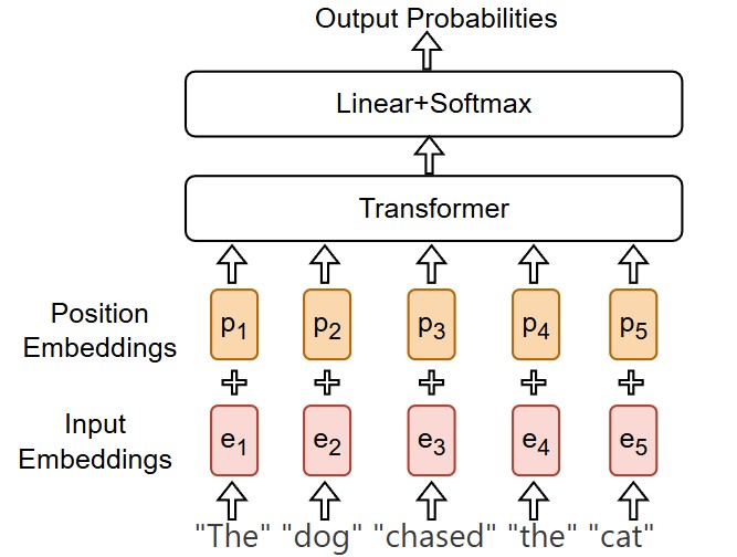
Imagine trying to understand the difference between “The dog chased the cat” and “The cat chased the dog.” The words are the same, but their order completely changes the meaning. To solve this, Transformers need a way to understand the position of each token in a sequence. This is where positional embeddings come in. They are vectors that provide the model with information about the order of tokens.
There are two primary families of positional embeddings: Absolute Positional Embeddings (APE) and Relative Positional Embeddings (RPE). Let us explore both.
Absolute Positional Embeddings (APE): Giving Each Word a Fixed Address
The most straightforward way to inform the model about word order is to assign a unique, fixed “address” to each position in the sequence. This is the core idea behind Absolute Positional Embeddings.
Intuition: The Bookshelf Analogy
Imagine a long bookshelf with numbered slots. Each book on the shelf has its own content (its meaning), but its position is defined by the slot number it occupies. APE works similarly. We create a unique embedding for each position (slot 1, slot 2, etc.) and add this positional embedding to the token’s own embedding (the book’s content). This combined embedding tells the model not only what a word is but also where it is in the sentence.
The Technical Details: Sinusoidal Embeddings
The original Transformer paper, “Attention Is All You Need,” introduced a clever way to create these absolute positional embeddings using sine and cosine functions of different frequencies.
For a token at position \(pos\) in a sequence, its positional embedding \(PE\) is a vector of the same dimension as the token embedding, \(d_{model}\). Each element of this vector is calculated as follows:
$$
PE_{(pos, 2i)} = \sin(pos / 10000^{2i/d_{model}})
$$
$$
PE_{(pos, 2i+1)} = \cos(pos / 10000^{2i/d_{model}})
$$
Where:
- \(pos\) is the position of the token in the sequence (e.g., 0, 1, 2, …).
- \(i\) is the dimension index within the embedding vector (from 0 to \(d_{model}/2\)).
- \(d_{model}\) is the dimensionality of the embedding.
To build further intuition, it helps to look at the sinusoidal positional embedding as a literal sine wave.
Consider the sine component used for the even dimensions:
$$
PE_{(pos, 2i)} = \sin\left(\frac{pos}{10000^{2i/d_{model}}}\right)
$$
This has the same form as a standard sinusoidal function:
$$
y = \sin(\omega t + \phi)
$$
If we interpret:
- \(t\) as the position \(pos\),
- \(\phi = 0\) (no phase shift),
- and \(\omega = \frac{1}{10000^{2i/d_{model}}} = \frac{1}{B_i}\)
then each even dimension \(2i\) corresponds to a sine wave with its own angular frequency \(\omega\).
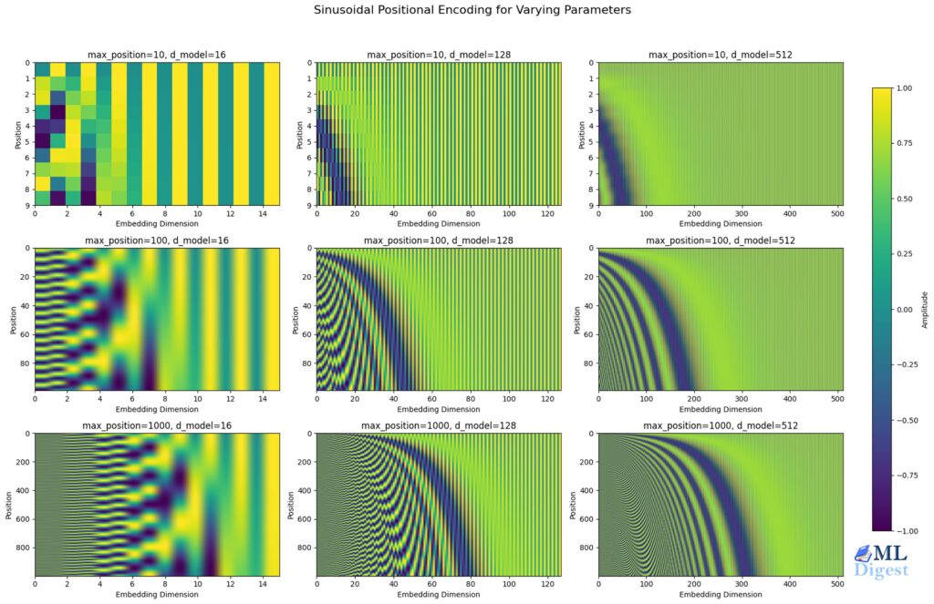
How Frequency Changes Across Dimensions?
As the dimension index \(i\) increases, the exponent \(2i/d_{model}\) increases, which makes \(10000^{2i/d_{model}}\) larger, and therefore \(\omega\) smaller. In other words:
- Lower dimensions (small \(i\)) have higher angular frequency
The sine wave oscillates rapidly as \(pos\) increases, so the positional values change a lot between adjacent positions. - Higher dimensions (large \(i\)) have lower angular frequency
The sine wave changes slowly with \(pos\), so the positional values change only slightly between adjacent positions.
This means that within a single positional embedding vector:
- The first few dimensions capture high-frequency, fine-grained positional changes.
- The later dimensions capture low-frequency, coarse positional trends.
You can think of this as each token position being described using a mixture of “short-range detail” and “long-range structure” signals, all packed into the same vector.
Why this complex formula?
This sinusoidal approach has several elegant properties:
- Uniqueness: It generates a unique positional embedding for each timestep.
- Constant Offset Relationship: For any fixed offset \(k\), the positional embedding at \(pos+k\) can be represented as a linear transformation of the embedding at \(pos\). This property makes it easy for the model to learn relative positions.
- Extrapolation: It can theoretically handle sequences longer than those seen during training, as the sinusoidal functions can extend indefinitely.
A detailed analysis of these properties can be found in these blog posts: article0, article1, article2.
Code in Practice: PyTorch Implementation
Here is how you can generate and apply APE in PyTorch.
import torch
import torch.nn as nn
import math

class AbsolutePositionalEmbedding(nn.Module):
    def __init__(self, d_model, max_len=5000):
        super().__init__()
        self.d_model = d_model

        # Create a positional encoding matrix
        pe = torch.zeros(max_len, d_model)

        # Create a tensor for positions (0, 1, 2, ..., max_len-1)
        position = torch.arange(0, max_len, dtype=torch.float).unsqueeze(1)

        # Create the division term for the denominator
        div_term = torch.exp(torch.arange(0, d_model, 2).float() * (-math.log(10000.0) / d_model))

        # Calculate the sinusoidal values
        pe[:, 0::2] = torch.sin(position * div_term)
        pe[:, 1::2] = torch.cos(position * div_term)

        # Register 'pe' as a buffer. Buffers are part of the model's state
        # but are not considered parameters to be trained.
        self.register_buffer('pe', pe.unsqueeze(0))

    def forward(self, x):
        """
        Args:
            x: Tensor of shape [batch_size, seq_len, d_model]
        """
        # Add the positional encoding to the input tensor
        # x.size(1) is the sequence length
        x = x + self.pe[:, :x.size(1)]
        return x

# Example Usage
d_model = 512
seq_len = 100
batch_size = 10

# Create dummy token embeddings
token_embeddings = torch.randn(batch_size, seq_len, d_model)

# Initialize and apply positional embeddings
pos_encoder = AbsolutePositionalEmbedding(d_model)
final_embeddings = pos_encoder(token_embeddings)

print("Shape of token embeddings:", token_embeddings.shape)
print("Shape of final embeddings after adding APE:", final_embeddings.shape)Limitations of APE
While effective, APE has its drawbacks. It assigns an absolute position, which might not be the most crucial piece of information. Often, the relative distance and relationship between words (e.g., “how far apart are ‘cat’ and ‘chased’?”) are more important for the attention mechanism. Furthermore, for very long sequences, the fixed nature of APE might struggle to generalize.
Relative Positional Embeddings (RPE): It’s All About Relationships
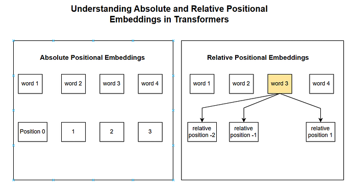
Relative Positional Embeddings were developed to address the limitations of APE. The core idea is that the attention between two tokens should depend on their relative distance, not their absolute positions.
Intuition: A Conversation in a Hallway
Imagine you are in a long hallway talking to someone. Your ability to hear them depends on the distance between you, not where you both are standing in the hallway. If you are 5 feet apart, it does not matter if you are at the beginning, middle, or end of the hallway. RPE brings this concept to Transformers. It modifies the self-attention mechanism to consider the pairwise distance between tokens when calculating attention scores.
The Technical Details: Modifying Self-Attention
RPE does not add positional information to the input embeddings. Instead, it injects relative position information directly into the attention calculation. A common approach, introduced in papers like the Transformer-XL, involves modifying the attention score formula.
The standard attention score between a query \(q_m\) (at position \(m\)) and a key \(k_n\) (at position \(n\)) is:
$$
\text{score}(m, n) = q_m^\top k_n
$$
With RPE, this is extended to include relative position information:
$$
\text{score}(m, n) = q_m^\top k_n + q_m^\top R_{m-n}
$$
Where: \(R_{m-n}\) is a learnable embedding representing the relative distance \(m-n\) between the query token and the key token.
For a token at position \(m\), with word embedding \(e_m\) and positional embedding \(p_m\), we have
$$
q_m = W_q (e_m + p_m),
\quad
k_n = W_k (e_n + p_n)
$$
Expanding again,
$$
q_m^\top k_n = \underbrace{e_m^\top W_q^\top W_k e_n}_{\text{content–content}} + \underbrace{\big(e_m^\top W_q^\top W_k p_n + p_m^\top W_q^\top W_k e_n\big)}_{\text{content–position}} +\underbrace{p_m^\top W_q^\top W_k p_n}_{\text{position–position}}
$$
The first two groups (content–content and content–position) are content dependent and can be thought of as the usual content-based attention. The last group is where relative geometry enters.
By introducing the learnable parameters (\(u, v\)) and splitting \(W_k\) into two matrices, one for input token (embedding – \(e\)) and one for position (\(R\)), we can rewrite the above as
$$ q_m^\top k_n = e_m^\top W_q^\top W_{k,e} e_n + e_m^\top W_q^\top W_{k,R} R_{m-n} + u^\top W_{k,e} e_n + v^\top W_{k,R} R_{m-n} $$
Note that \(R_{m-n}\) is a sinusoid encoding matrix without learnable parameters, similar to APE, but indexed by relative distance \((m-n)\) rather than absolute position. This means the positional interaction term \(p_m^\top W_q^\top W_k p_n\) now depends only on the relative distance \((m – n)\), not on the absolute positions \(m\) and \(n\).
Deriving Relative Terms from Sinusoidal APE
To connect this with relative positions, we examine one sinusoidal pair and then generalize.
Step 1: One Sin–Cos Pair Gives a Relative-Term Only
For a single frequency band \(B_i\), you showed that
$$ \mathbf{p}_m=\begin{bmatrix}\sin\left(\frac{m}{B_i}\right)\\\cos\left(\frac{m}{B_i}\right)\end{bmatrix},\quad\mathbf{p}_n=\begin{bmatrix}\sin\left(\frac{n}{B_i}\right)\\\cos\left(\frac{n}{B_i}\right)\end{bmatrix}, $$
and with \(W_q = W_k = I\),
$$
\mathbf{p}_m^\top \mathbf{p}_n
= \cos\left(\frac{m-n}{B_i}\right).
$$
This is already a purely relative quantity: it depends only on the difference \((m – n)\), not on \(m\) and \(n\) separately. So for that band,
$$
\text{score}_i(m, n)
\;\propto\; \cos\left(\frac{m-n}{B_i}\right)
\;=\; f_i(m-n),
$$
for some function \(f_i\) of the relative displacement.
Step 2: Stack All Frequency Bands → Sum of Relative Terms
In the full sinusoidal positional embedding of dimension \(d_{\text{model}}\), you concatenate these 2D sin–cos blocks across many frequencies \(\{B_i\}_{i=1}^{d_{\text{model}}/2}\):
$$
p_m =
\begin{bmatrix}
\sin\left(\frac{m}{B_1}\right)\
\cos\left(\frac{m}{B_1}\right)\
\vdots\
\sin\left(\frac{m}{B_{d_{\text{model}}/2}}\right)\
\cos\left(\frac{m}{B_{d_{\text{model}}/2}}\right)
\end{bmatrix}.
$$
Then, still with \(W_q = W_k = I\) for clarity, the position–position interaction becomes
$$ p_m^\top p_n = \sum_{i=1}^{d_{\text{model}}/2} \left[ \sin\left(\frac{m}{B_i}\right)\sin\left(\frac{n}{B_i}\right) + \cos\left(\frac{m}{B_i}\right)\cos\left(\frac{n}{B_i}\right) \right] = \sum_{i=1}^{d_{\text{model}}/2} \cos\left(\frac{m-n}{B_i}\right). $$
Define the relative offset \(\Delta = m – n\). Then
$$ p_m^\top p_n = \sum_{i=1}^{d_{\text{model}}/2} \cos\left(\frac{\Delta}{B_i}\right) \;=\; g(\Delta), $$
for some deterministic function \(g\) that depends only on the relative distance \(\Delta\). This is the mathematical core: *the positional dot product is a function of the relative distance only*.
The learnable parameters in \(u\), \(v\), \(W_q\), \(W_{k,e}\) and \(W_{k,R}\) allow the model to adaptively weight and mix these relative signals, leading to the final form where the position–position term can be approximated by a learned relative position embedding lookup.
This can be reparameterized using a learnable embedding \(R_{m-n}\) instead of a fixed sinusoidal interaction, and attach it to the query:
$$
\text{position–position term}
\;\approx\;
q_m^\top R_{m-n}.
$$
The full attention score thus becomes
$$ \text{score}(m, n) = q_m^\top k_n + q_m^\top R_{m-n}, $$
where the first part captures content-based similarity and the second part explicitly encodes the learned effect of the relative offset \(m-n\).
This means we are creating embeddings for relative distances (e.g., -1, 0, 1, 2, …). The model can then learn, for example, that a relative distance of “+1” (the next word) is particularly important.
A more sophisticated version from the T5 paper breaks this down further:
$$
\text{score}(i, j) = q_i^T k_j + b_{i-j}
$$
Here, \(b_{i-j}\) is a simple, learnable scalar (a bias) that is added to the attention score based on the relative distance. This is computationally simpler and has been shown to be very effective. The model learns a set of biases for a range of relative positions (e.g., from -128 to +128) and adds the corresponding bias to each attention score.
Code in Practice: T5-style Relative Attention Bias
Implementing RPE is more involved as it requires modifying the attention mechanism itself. Here is a conceptual implementation of the T5-style relative attention bias.
import torch
import torch.nn as nn

class T5RelativeAttention(nn.Module):
    def __init__(self, num_heads, max_relative_position=128):
        super().__init__()
        self.num_heads = num_heads
        self.max_relative_position = max_relative_position

        # Create a learnable embedding table for relative position biases.
        # We need embeddings for distances from -max_relative_position to +max_relative_position,
        # but we can map them to a smaller table.
        self.relative_attention_bias = nn.Embedding(2 * max_relative_position, num_heads)

    def forward(self, seq_len):
        """
        Generates the bias tensor to be added to the attention scores.

        Args:
            seq_len: The length of the sequence.

        Returns:
            A bias tensor of shape [1, num_heads, seq_len, seq_len]
        """
        # Create a matrix of relative positions
        # context_position are columns (keys), memory_position are rows (queries)
        context_position = torch.arange(seq_len, dtype=torch.long)[:, None]
        memory_position = torch.arange(seq_len, dtype=torch.long)[None, :]
        relative_position = memory_position - context_position

        # Clip the relative positions to be within the range [-max, max]
        # and shift them to be positive for embedding lookup (0 to 2*max-1)
        relative_position_bucket = relative_position + self.max_relative_position - 1
        relative_position_bucket = torch.clamp(relative_position_bucket, 0, 2 * self.max_relative_position - 2)

        # Look up the bias from the embedding table
        bias = self.relative_attention_bias(relative_position_bucket)

        # Reshape to [seq_len, seq_len, num_heads] and then permute
        # to [num_heads, seq_len, seq_len] to match attention matrix shape
        bias = bias.permute(2, 0, 1).unsqueeze(0)
        return bias

# In the attention mechanism, you would calculate this bias and add it
# to the qk_T scores before the softmax.

# qk_scores = torch.matmul(query, key.transpose(-1, -2))
# relative_bias = self.relative_attention.forward(seq_len)
# qk_scores_with_bias = qk_scores + relative_bias
# attention_probs = F.softmax(qk_scores_with_bias, dim=-1)APE vs. RPE: Which is Better?
- Simplicity: APE is simpler to implement, as it is a plug-and-play module that preprocesses the embeddings. RPE requires modifying the internals of the attention mechanism.
- Performance: For many tasks, RPE-based models like T5, DeBERTa, and Transformer-XL have shown superior performance, especially on tasks requiring a nuanced understanding of long-range dependencies. The intuition is that relative positions are often more meaningful than absolute ones.
- Extrapolation: RPE naturally handles sequences of varying lengths better than the most basic form of APE, as it focuses on local, relative distances.
- Hybrid Approaches: Some modern architectures, like DeBERTa, use a combination of both absolute and relative positional information to get the best of both worlds.
Conclusion
Positional embeddings are a foundational component of the Transformer architecture, solving the critical problem of permutation invariance.
- Absolute Positional Embeddings (APE) provide a fixed, unique “address” for each token, typically by adding a sinusoidal signal to the token embedding. It is simple and effective but can be rigid.
- Relative Positional Embeddings (RPE) encode the distance between pairs of tokens directly into the attention mechanism, making the model focus on relationships rather than fixed locations. It is more complex but often yields better performance and generalization.
The choice between them depends on the specific application, but the trend in state-of-the-art models has been a move towards the more dynamic and flexible relative positional schemes.

Happy is a seasoned ML professional with over 15 years of experience. His expertise spans various domains, including Computer Vision, Natural Language Processing (NLP), and Time Series analysis. He holds a PhD in Machine Learning from IIT Kharagpur and has furthered his research with postdoctoral experience at INRIA-Sophia Antipolis, France. Happy has a proven track record of delivering impactful ML solutions to clients.
Subscribe to our newsletter!