In tabular machine learning, the winning recipe is often not a flashy architecture but strong features plus a fast, reliable learner. Gradient Boosting Machines (GBMs) have dominated that setting for years. XGBoost pushed the field forward with careful engineering and regularization. LightGBM pushed it further by asking a sharper question: how do we preserve most of that accuracy while cutting training cost on large, high-dimensional datasets?
Enter LightGBM.
Imagine you’re building a Lego castle. A level-wise approach builds one full layer at a time, keeping everything balanced before moving upward. LightGBM is more opportunistic: it looks for the branch of the structure where the next block will create the biggest payoff and keeps building there first. That best-first intuition explains one visible part of LightGBM’s behavior. The full speed story also includes histogram-based training, selective sampling, and feature bundling.
This article is a practical guide to understanding, implementing, and tuning LightGBM. We will start with the foundations, then move through the architectural choices that make LightGBM distinct, and finally cover the workflow most teams actually need: build a baseline, tune the high-leverage parameters, interpret the model, and decide whether LightGBM is the right tool for the job.
1. Foundations and Context
Before we can appreciate LightGBM’s innovations, we need to understand the giants on whose shoulders it stands.
1.1 Decision Trees and Ensemble Methods
- Decision Trees (CART):
At its core, a decision tree is like a flowchart of questions used to classify or predict an outcome. Starting at the root, the tree splits data based on feature values. For example, “Isage> 30?” or “Iscity== ‘New York’?”. Each split leads to a new node, and this continues until we reach a terminal node (a “leaf”), which provides the final prediction. - Ensemble Methods:
A single tree can be prone to overfitting. Ensemble methods combine multiple weak learners (like decision trees) to create a single, powerful model.- Bagging (e.g., Random Forest): This method builds multiple independent decision trees, each trained on a bootstrap sample (random sampling with replacement) of the data, and a random subset of features at each split. The final prediction is an average (for regression) or a majority vote (for classification) of all the trees. It’s a parallel, democratic process.
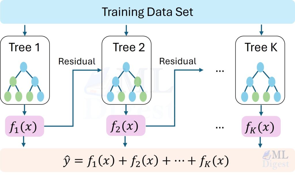
- Boosting: This is a sequential process. It starts with a simple model, identifies its errors, and builds a new model specifically to correct those errors. Each new tree focuses on the mistakes of the previous ones. It’s like a team of specialists, where each new member is trained to fix the problems the previous one missed.
1.2 The Evolution of Gradient Boosting
- Gradient Boosting Machine (GBM):
This is the foundational algorithm. Instead of just correcting “errors,” it uses a more sophisticated method: gradients. In simple terms, for each data point, it calculates the direction of the error (the gradient of the loss function) and trains the next tree to predict this gradient. By moving in the opposite direction of the gradient, it systematically minimizes the overall error. - XGBoost (eXtreme Gradient Boosting):
XGBoost was a game-changer. It improved upon the standard GBM with several key innovations:- Regularization: It added L1 and L2 regularization terms to the loss function, penalizing complex models to prevent overfitting.
- Sparsity Handling: It learned how to handle missing values automatically.
- Level-wise Tree Growth: Originally, it built trees level by level, ensuring all nodes at a given depth are split before moving to the next depth. This is thorough but can be slow (Note: Modern XGBoost also supports leaf-wise growth).
- Motivation for LightGBM:
When LightGBM was introduced, XGBoost’s exact split-finding and data handling could be expensive on very large or high-dimensional datasets. LightGBM was built to reduce that cost through histogram-based training, leaf-wise split selection, and additional sampling and feature-bundling tricks. Its speed advantage did not come from one idea alone; it came from several engineering decisions working together. (Note: Over time, the libraries have converged; XGBoost now also uses histogram-based training by default and supports leaf-wise growth and native categorical processing).
2. LightGBM Core Architecture and Concepts
LightGBM’s speed comes from several design choices working together, not from one isolated trick. We can separate it into three layers:
- the boosting algorithm, which decides what the next tree should correct,
- the histogram engine, which makes split search cheap, and
- scale-oriented optimizations such as GOSS, EFB, and native categorical handling, which reduce the amount of work on large datasets.
With that framing in place, the rest of the architecture becomes much easier to follow.
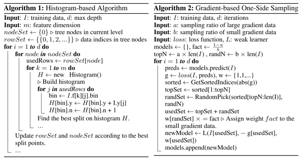
2.1 Histogram-Based Learning
This is the foundational speed innovation in LightGBM — the mechanism that makes every other optimization practical at scale.
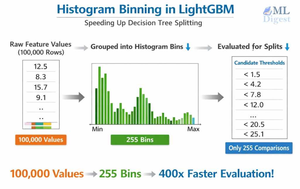
Traditional exact split-finding (used in early gradient boosting implementations) sorts all feature values for each split candidate. For $n$ rows and $d$ features that amounts to $O(n \times d)$ comparisons per tree level — very expensive on large datasets.
LightGBM instead pre-bins every continuous feature into at most $k$ discrete buckets before training begins (default: 255 bins). Split-finding then operates on histograms rather than raw sorted values:
- Pre-binning: Each continuous value is mapped to an integer bin index. Memory footprint drops sharply — a 64-bit float becomes an 8-bit integer.
- Histogram construction: For each tree node, accumulate the sum of gradients and hessians into a histogram over the bins — $O(n)$ per feature.
- Split evaluation: Scan the histogram left-to-right evaluating the gain for each candidate threshold — $O(k)$ per feature. Since $k \ll n$ for large datasets, this is orders of magnitude faster than sorting.
- Histogram subtraction trick: The parent histogram equals the left child’s histogram plus the right child’s histogram. After computing the smaller child directly (scanning fewer data points is cheaper), the larger child’s histogram is obtained by subtraction — cutting construction cost roughly in half.
Trade-offs:
- Speed and memory: Major gains over exact methods, especially when $n \gg k$.
- Mild approximation: Binning introduces slight discretization. In practice, 255 bins captures most real-world feature distributions well, and the coarser granularity can mildly improve generalization by smoothing noise in extreme feature values.
Key parameter: max_bin (default: 255). Reducing it (e.g., to 63–127) speeds up training on very large datasets with a minor accuracy trade-off. Rarely worth increasing beyond the default.
2.2 The Leaf-wise Tree Growth Strategy
This is one of the most visible differences between LightGBM and traditional level-wise boosting libraries.
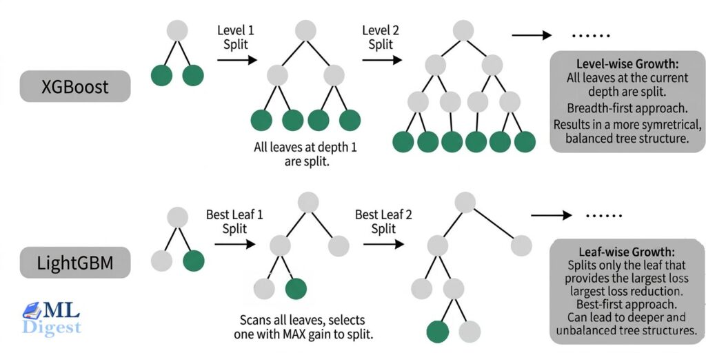
- Level-wise (XGBoost/Traditional): Grows the tree layer by layer. It’s a breadth-first search.
- Leaf-wise (LightGBM): Instead of growing horizontally, it grows vertically. It scans all the current leaves and splits the one that will produce the largest reduction in loss. It’s a best-first search.
- Trade-offs:
- Better loss reduction per split: Leaf-wise growth often reaches lower training loss with the same number of leaves because it always expands the most promising leaf.
- Potential speed gains: In practice this can be faster, especially when combined with LightGBM’s other optimizations, because the algorithm spends effort where it matters most.
- Higher overfitting risk: The same aggressive focus can create very deep, highly specific branches, especially on smaller or noisy datasets. This is why
num_leaves,max_depth, andmin_child_samplesmatter so much in LightGBM.
Mini Pseudocode Comparison (conceptual, simplified):
Level-wise (breadth-first):
queue = [root]
while depth < max_depth:
    next_level = []
    for node in queue:
        best_split = find_best_split(node)
        apply(best_split)
        next_level.extend(node.children)
queue = next_levelLeaf-wise (best-first):
leaves = [root]
while num_leaves < limit:
    # Evaluate potential gain for splitting each leaf
    candidate = argmax_over(leaves, gain_if_split(leaf))
    perform_split(candidate)
update(leaves)Key control parameters for beginners:
num_leaves: Hard cap on how many terminal leaves the algorithm can create (primary complexity dial). Start with 31 (default); adjust after baseline.max_depth: Safety net; set (e.g., 6–10) if you observe overfitting or extremely deep trees when inspecting.min_child_samples: Prevents splits creating leaves with too few rows—raise this (e.g., 50–100) when dataset is small or noisy.
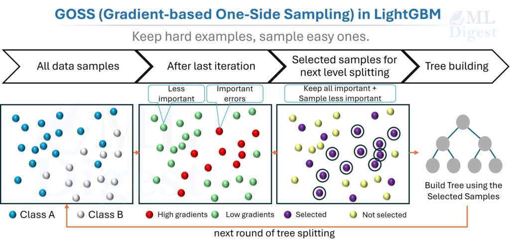
2.3 Gradient-based One-Side Sampling (GOSS)
- Concept: In boosting, not all data points are equally important. Instances with large gradients (i.e., those that are poorly predicted) are the most valuable for training the next learner. Instances with small gradients are already well-trained.
- GOSS Mechanism: Instead of using all data points to calculate the next split, GOSS keeps more of the high-gradient examples and fewer of the low-gradient ones:
- It keeps all the instances with large gradients.
- It takes a random sample of the instances with small gradients.
- To maintain the same data distribution, it amplifies the contribution of the small-gradient data by a constant factor during training.
- Important practical note: GOSS is one of LightGBM’s signature techniques, but it is not applied by default. The default
boosting_type='gbdt'uses standard gradient boosting without GOSS sampling. To enable it, explicitly setboosting_type='goss'(ordata_sample_strategy='goss'in LightGBM v4+). Once enabled, the sampling process is handled automatically, but advanced users can tune it withtop_rate(the fraction of large-gradient instances to retain, default:0.2) andother_rate(the fraction of small-gradient instances to randomly sample, default:0.1). Settingtop_rate + other_rateto be too large effectively negates the sampling benefit, while settingother_ratetoo low can introduce variance — the defaults are a good starting point for most workloads.
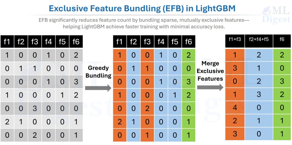
2.4 Exclusive Feature Bundling (EFB)
What problem does EFB solve? High-dimensional datasets are often very sparse. Most entries are zero, and many features are near-mutually exclusive — they rarely carry non-zero values simultaneously. EFB exploits this by bundling such features together, reducing the effective dimensionality without losing information.
EFB asks a simple question: if two features almost never “light up” together, why keep scanning them as separate columns? Instead, LightGBM bundles them together so the model has fewer effective features to process.
Two key subproblems: EFB is easier to understand if we split it into two smaller questions:
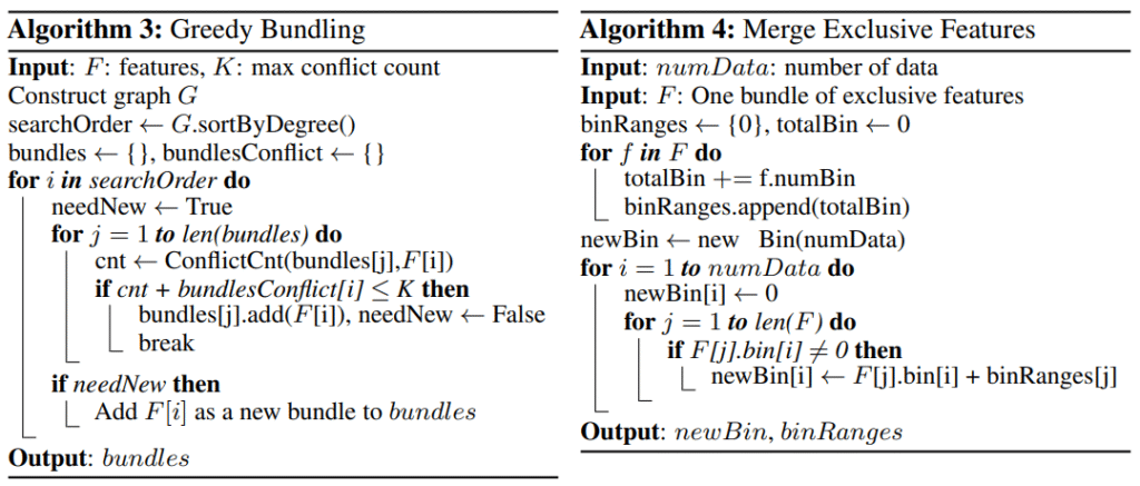
- Greedy Bundling: Which features should be bundled together?
- Merge Exclusive Features: How do bundled features share one column without becoming ambiguous?
Click here to see details of EFB process.
What is a conflict?
Before bundling, we need a way to measure whether two features are compatible.
A conflict happens when two features are non-zero in the same row.
Example:
Feature A: [0, 1, 0, 0]
Feature B: [1, 0, 0, 1]
These do not conflict, because there is no row where both are non-zero at the same time.
Now compare that with:
Feature A: [0, 1, 0, 0]
Feature C: [0, 1, 1, 0]
A and C do conflict, because both are non-zero in the second row.
Intuitively, low-conflict pairs are good bundling candidates. High-conflict pairs are not.
Part A: Greedy Bundling (which features go together?)
LightGBM models this as a graph-coloring-style problem:
- Nodes = features
- Edges = conflicts between features
If two features conflict heavily, imagine drawing a thick edge between them. Bundling then becomes similar to assigning colors to nodes: features with compatible conflict patterns can share the same color, and each color corresponds to one bundle.
The workflow is conceptually:
- Build a conflict matrix: Compare every pair of features and count how many rows contain non-zero values for both.
- Compute a conflict degree for each feature: Sum how much each feature conflicts with the rest. Features with larger conflict degree are harder to place.
- Sort features by conflict degree: Handle the hardest-to-place features first.
- Choose a conflict threshold $K$: This is the maximum amount of conflict you are willing to tolerate inside one bundle.
- Process features greedily:
- Try to place the current feature into an existing bundle.
- If its added conflict with that bundle stays at or below $K$, place it there.
- Otherwise, create a new bundle.
This is called greedy bundling because it makes the best immediate placement decision at each step instead of searching for the global optimum.
The important intuition is that EFB does not need a perfect global solution. It just needs a fast, good-enough bundling strategy that keeps conflicts low. That is exactly why the greedy approach works well in practice.
One practical note: in the EFB paper this tolerance is expressed as a maximum conflict count $K$. In LightGBM’s implementation, this is mostly an internal heuristic rather than a parameter most users tune directly; the code derives a small allowed conflict count from the sampled rows used during bin construction rather than exposing a commonly used max_conflict_rate knob.
Part B: Merge Exclusive Features (how do bundled features become one column?)
Once LightGBM decides which features belong together, it still needs to encode them into one bundled feature without mixing them up.
The trick is to give each original feature its own bin range inside the bundle.
Remember that LightGBM already bins continuous features into discrete integer bins. EFB operates on those bins, not on raw floating-point values. So the merge step is really: shift each feature’s bin IDs by an offset so their value ranges do not overlap.
Here is the beginner-friendly version:
- Feature A uses one bin range.
- Feature B is shifted by an offset so it occupies a different range.
- Feature C is shifted again, and so on.
Example after binning:
Feature Acan take bins0, 1, 2Feature Bcan take bins0, 1, 2, 3
If we reserve bins 0-2 for A, then we can shift B so its active bins become 3-5.
| Original row | A bin | B bin | Merged value |
|---|---|---|---|
| Row 1 | 2 | 0 | 2 |
| Row 2 | 0 | 1 | 3 |
| Row 3 | 0 | 3 | 5 |
| Row 4 | 0 | 0 | 0 |
| Row 5 | 1 | 0 | 1 |
Now one bundled column can represent either feature unambiguously:
- merged value
2means “this came fromA” (Feature A was in bin 2) - merged value
3or5means “this came fromB” (Feature B was in bin 1 or 3, respectively, shifted by +2) - merged value
0means both features are at their zero/default value — neither was active in that row
The same idea is even easier to see with one-hot features. Suppose is_city_A, is_city_B, and is_city_C are mutually exclusive columns:
is_city_A | is_city_B | is_city_C | bundled feature |
|---|---|---|---|
| 1 | 0 | 0 | 1 |
| 0 | 1 | 0 | 2 |
| 0 | 0 | 1 | 3 |
| 0 | 0 | 0 | 0 |
Three sparse columns become one sparse column, with no loss of meaning.
What about conflicts during merging?
The cleanest case is when each row contributes at most one non-default value to the bundle. If two bundled features are non-zero in the same row, that row is a conflict.
Too many such rows would break the nice one-feature-per-range picture, which is why greedy bundling tries to keep bundle conflicts below a threshold. In practice, LightGBM can tolerate a small amount of conflict and still get most of the dimensionality reduction benefit. The general rule is simple: the rarer the conflicts, the safer and more effective the bundle.
Why EFB matters in practice:
By reducing the effective number of features that LightGBM must scan during split finding, EFB can provide large speed and memory gains with little or no meaningful accuracy loss. It is especially helpful when:
- the dataset is high-dimensional,
- many features are sparse,
- one-hot encoding exploded the number of columns, and
- feature count, rather than row count, is the main bottleneck.
An interesting video on EFB can be found here: LightGBM EFB Explained.
2.5 Efficient Categorical Feature Handling
- Traditional Approach: The standard way to handle categorical features is one-hot encoding. This creates many sparse features, which is computationally expensive for tree-based models.
- LightGBM Approach: LightGBM can handle categorical features directly. Rather than blindly expanding every category into separate one-hot columns, it uses a smarter split-finding strategy: it sorts category values by their mean gradient (which approximates sorting by the mean target value) and then searches for the optimal split threshold along that sorted order. This reduces what would otherwise be an exponential search over all possible category partitions into a single linear scan — offering both speed benefits and potentially better splits for medium-cardinality variables. In many tabular problems this is both faster and more memory-friendly than one-hot encoding. For very high-cardinality columns, benchmark carefully: CatBoost, target encoding, or ordinal encoding may be more stable depending on the problem.
2.6 How Gradient Boosting Actually Updates the Model
We try to approximate an unknown target function $F^*(x)$ by adding small corrective functions (trees) sequentially:
- Start with a simple constant prediction: $F_0(x) = \arg\min_c \sum_i L(y_i, c)$
- At iteration $m$, compute the first and second-order derivatives of the loss function (gradients $g_i$ and hessians $h_i$) with respect to the current predictions $F_{m-1}(x_i)$.
- Fit a regression tree structure that optimizes exactly these Newton steps. Using a second-order Taylor expansion of the loss function, LightGBM derives a closed-form solution for the optimal weight of each leaf:
$$ w_{leaf} = – \frac{\sum_{i \in leaf} g_i}{\sum_{i \in leaf} h_i + \lambda} $$ - Update the model predictions for each data point:
$$ F_m(x) = F_{m-1}(x) + \eta \cdot \text{Tree}_m(x) $$
Where $\eta$ is the learning rate, and $\lambda$ is an L2 regularization term.
You do not need to memorize the equations. The important idea is that each tree is a corrective brush stroke guided by gradients, while the hessians help scale how aggressive that correction should be. A smaller $\eta$ makes each stroke gentler, so you usually need more rounds, but the optimization path is often smoother.
2.7 When LightGBM Is a Strong Choice
Reach for LightGBM when most of the following are true:
- Your data is tabular and mostly fits into rows and columns.
- You care about fast iteration and strong baseline accuracy.
- Your feature set includes missing values, numeric fields, and categorical variables.
- You need a model that is usually easier to train than a deep neural network.
Be more cautious when:
- The dataset is tiny and a simpler model may generalize better.
- Categories are extremely high-cardinality and CatBoost may be a better fit.
- The main signal lives in raw text, images, or sequential structure rather than engineered table features.
Common failure modes to watch for:
- aggressive
num_leaveson small or noisy data, - leakage hidden inside engineered features,
- inappropriate validation strategy for time series or grouped data, and
- unstable behavior from rare or poorly handled categorical values.
LightGBM is also competitive for time-series forecasting when combined with engineered lag features, rolling statistics, and calendar features. Because LightGBM treats each row independently, temporal structure must be captured explicitly in the feature engineering stage — but when done well, this approach is competitive with deep learning on many tabular time series benchmarks (e.g., M5 competition).
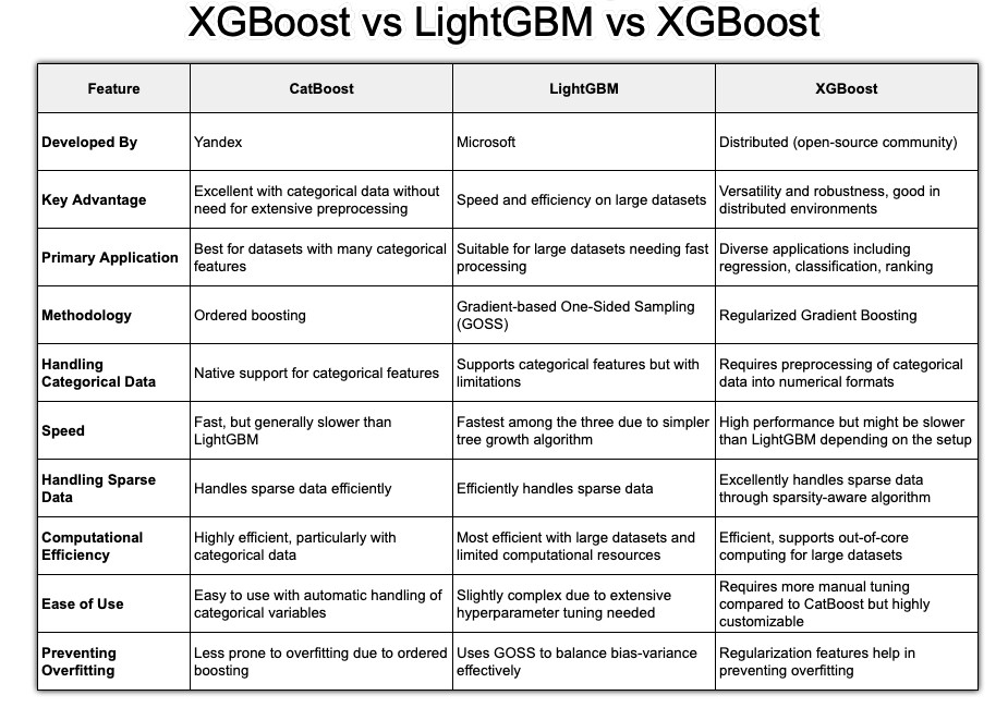
A quick comparison of LightGBM with other popular algorithms is given below:
3. Practical Implementation of LightGBM
Let’s translate theory into practice with Python.
3.1 Setup and Data Preparation
- Installation:
pip install lightgbm numpy pandas scikit-learn - Data Format: The Scikit-learn API is the easiest place to start. When the dataset gets larger or you need tighter control over weights, categorical columns, or repeated training runs, the native
lightgbm.Datasetobject becomes more attractive. The main practical rule is simple: choose a validation split that matches the data-generating process. Use random or stratified splits for i.i.d. tabular data, but use chronological splits for time series and grouped splits when rows from the same entity should not leak across train and validation.
import lightgbm as lgb
import pandas as pd
from sklearn.model_selection import train_test_split

# Sample data
data = {
    'feature1': [1, 2, 3, 4, 5, 6, 7, 8, 9, 10],
    'feature2': [10, 9, 8, 7, 6, 5, 4, 3, 2, 1],
    'category': ['A', 'B', 'A', 'C', 'B', 'C', 'A', 'A', 'B', 'C'],
    'target': [0, 1, 0, 1, 0, 1, 0, 0, 1, 1]
}
df = pd.DataFrame(data)
df['category'] = df['category'].astype('category') # Crucial step!

X = df.drop('target', axis=1)
y = df['target']

X_train, X_val, y_train, y_val = train_test_split(X, y, test_size=0.2, random_state=42, stratify=y)

# Create LightGBM Dataset objects
lgb_train = lgb.Dataset(X_train, y_train)
lgb_val = lgb.Dataset(X_val, y_val, reference=lgb_train)Memory and categorical tips:
- Converting text categories to
categorydtype drastically reduces memory and enables native categorical splits. - For large data, you can pass
categorical_featureexplicitly (list of column names or indices) to ensure correct treatment:
categorical_cols = ['category']
lgb_train = lgb.Dataset(X_train, y_train, categorical_feature=categorical_cols)
lgb_val = lgb.Dataset(X_val, y_val, reference=lgb_train, categorical_feature=categorical_cols)- Missing values (
NaN) need no preprocessing; LightGBM learns optimal default direction. - Keep the category vocabulary consistent between training and inference. Native categorical support helps only if the preprocessing layer preserves the same meaning for each category value.
- Use
lgb.Datasetwhen: (a) data is large, (b) you need finer control (weights, categorical features), (c) you want faster repeated training. Otherwise, start with scikit-learn API for simplicity.
3.2 Basic Model Training (Python API)
The native API is often more flexible and can be more efficient in repeated or larger-scale training workflows.
# Define parameters
params = {
    'objective': 'binary',
    'metric': 'auc',
    'boosting_type': 'gbdt',
    'num_leaves': 31,
    'learning_rate': 0.05,
    'feature_fraction': 0.9
}

# Train the model
gbm = lgb.train(params,
                lgb_train,
                num_boost_round=100,
                valid_sets=[lgb_val],
                callbacks=[lgb.early_stopping(stopping_rounds=10)])

# Make predictions
y_pred_proba = gbm.predict(X_val, num_iteration=gbm.best_iteration)Key Concepts:
num_boost_round: The maximum number of trees to build.early_stopping: This callback monitors the performance on the validation set (lgb_val) and stops training if the metric (aucin this case) doesn’t improve for10consecutive rounds. This is the best way to choose the number of trees and prevent overfitting.
3.3 Scikit-learn API (Beginner Friendly)
If you prefer the familiar fit/predict interface:
Classification example:
from lightgbm import LGBMClassifier

clf = LGBMClassifier(
    objective='binary',
    learning_rate=0.05,
    n_estimators=500,      # upper bound; early stopping will cut it
    num_leaves=31,
    random_state=42
)

clf.fit(
    X_train, y_train,
    eval_set=[(X_val, y_val)],
    eval_metric='auc',
    callbacks=[lgb.early_stopping(25), lgb.log_evaluation(period=0)],
)

proba = clf.predict_proba(X_val)[:, 1]
preds = clf.predict(X_val)
print("Best iteration used:", clf.best_iteration_)Regression example:
from lightgbm import LGBMRegressor

reg = LGBMRegressor(
    objective='regression',
    learning_rate=0.05,
    n_estimators=800,
    num_leaves=63,
    random_state=42
)

reg.fit(
    X_train, y_train,
    eval_set=[(X_val, y_val)],
    eval_metric='l2',  # mean squared error
    callbacks=[lgb.early_stopping(30), lgb.log_evaluation(period=0)],
)

preds = reg.predict(X_val)
print("Best iteration used:", reg.best_iteration_)Notes:
- Set a generous
n_estimatorsthen rely oncallbacks=[lgb.early_stopping(n)]+ a validation metric to find the true stopping point. - Access
clf.best_iteration_to reuse the model appropriately (internally LightGBM already truncates). If you want to retrain on all data afterward, setn_estimators=clf.best_iteration_and fit again on combined train+val.
3.4 Cross-Validation Workflow
For more robust estimates of generalization performance — especially on smaller datasets or before a final retrain on the full data — use LightGBM’s built-in CV:
params = {
    'objective': 'binary',
    'metric': 'auc',
    'learning_rate': 0.05,
    'num_leaves': 31,
    'verbose': -1
}

cv_results = lgb.cv(
    params,
    lgb_train,
    num_boost_round=1000,
    nfold=5,
    callbacks=[lgb.early_stopping(50), lgb.log_evaluation(period=0)],
    seed=42
)

best_rounds = len(cv_results['valid auc-mean'])
print(f"Best num_boost_round: {best_rounds}")
print(f"CV AUC: {cv_results['valid auc-mean'][-1]:.4f} ± {cv_results['valid auc-stdv'][-1]:.4f}")After identifying best_rounds, retrain a final model on the full dataset (train + val combined) without a validation split:
final_model = lgb.train(
    params,
    lgb.Dataset(X, y),   # full data
    num_boost_round=best_rounds
)lgb.cv returns per-fold mean and standard deviation of the chosen metric at each boosting round. The last entry corresponds to the round selected by early stopping — use that as num_boost_round for your final production model.
3.5 Saving and Loading Models
# Save model
gbm.save_model('model.txt')

# Load model
loaded_model = lgb.Booster(model_file='model.txt')

# You can now use loaded_model to make predictions3.6 API Comparison: Native vs. Scikit-learn
| Feature | lightgbm.train() | LGBMClassifier.fit() |
|---|---|---|
| API type | Native LightGBM | sklearn-style |
| Ease of use | harder | easier |
| Flexibility | very high | moderate |
| Data format | Dataset required | NumPy / pandas |
| sklearn compatibility | no | yes |
| Custom training logic | best | limited |
4. Hyperparameter Optimization
This is where you unlock LightGBM’s full potential. Before diving in, here is a quick reference of the most important parameters:
| Parameter | Default | Effect | When to change |
|---|---|---|---|
num_leaves | 31 | Max leaves per tree (complexity) | Lower if overfitting; raise if underfitting |
learning_rate | 0.1 | Step size per boosting round | Lower (0.01–0.05) for smoother convergence |
n_estimators | 100 | Max boosting rounds | Set high; let early stopping decide |
min_child_samples | 20 | Min rows per leaf | Raise (50–200) for small/noisy data |
max_depth | -1 (unlimited) | Max tree depth | Set (6–12) as an overfitting safeguard |
feature_fraction | 1.0 | Fraction of features per tree | Lower (0.7–0.9) to reduce overfitting |
bagging_fraction | 1.0 | Fraction of rows per tree | Lower (0.7–0.9), pair with bagging_freq=1 |
lambda_l2 | 0.0 | L2 regularization | Try 1–10 if overfitting persists |
max_bin | 255 | Histogram bin count | Lower (63–127) to speed up very large data |
4.1 Tuning Priorities (The Big Three)
Focus on these first. They have the biggest impact on performance, and they are usually enough to produce a strong model. The common beginner mistake is tuning too many knobs at once and losing the causal link between a parameter change and the validation result.
num_leaves: This is the main complexity control for the tree. If you also setmax_depth = d, thennum_leavesshould generally stay at or below $2^d$. In practice, LightGBM often works better with a noticeably smaller value because leaf-wise growth can create very specialized branches.learning_rate(oreta): This determines the step size at each iteration. A smaller learning rate usually requires more trees, but it often gives you a smoother optimization path and better generalization.n_estimators(ornum_iterations): The number of boosting rounds. Think of this as an upper bound when you use early stopping, not as a value you need to guess precisely.
Beginner Stepwise Recipe:
- Start with:
learning_rate=0.05,num_leaves=31,n_estimators=1000, early stopping with 50 rounds (callbacks=[lgb.early_stopping(50)]). - Train and record best iteration and validation metric.
- If overfitting (train >> val), first raise
min_child_samples(e.g., 20 → 60) and lowernum_leaves(31 → 15–25). - If underfitting (both scores low), increase
num_leaves(31 → 63) OR decreaselearning_rateand increasen_estimators. - Once stable, do a finer sweep of
learning_rate(0.03, 0.05, 0.07) around best configuration.
Rule of thumb interplay:
num_leaves↑ often needsmin_child_samples↑ for stability.- Smaller
learning_rate→ largern_estimatorsbut potentially smoother generalization. - Use early stopping as your automatic guardrail—avoid guessing
n_estimators.
4.2 Overfitting Control (Regularization)
If your model is overfitting (validation score is much worse than training score), turn to these parameters.
- Tree Constraints:
max_depth: While LightGBM is leaf-wise, you can usemax_depthto limit the tree depth explicitly. This is a useful safeguard against extreme overfitting.min_child_samples(ormin_data_in_leaf): The minimum number of data points required in a leaf. A higher value prevents the tree from learning highly specific patterns for just a few data points.
- L1/L2 Regularization:
lambda_l1: L1 regularization. Applies soft-thresholding to leaf output values, discouraging extreme leaf scores. Unlike in linear models, this does not produce sparse feature weights—it regularizes the magnitude of the trees’ leaf outputs.lambda_l2: L2 regularization. The primary regularization term.
- Feature/Data Subsampling:
feature_fraction(orcolsample_bytree): Randomly selects a subset of features for each tree.bagging_fraction(orsubsample): Randomly selects a subset of data rows for each tree (without replacement). This must be used withbagging_freq.bagging_freq: The frequency (in iterations) to perform bagging. A value of1means bagging is performed at every iteration.
Starter Regularization Settings:
learning_rate: 0.05
num_leaves: 31
min_child_samples: 40   # raise for small/noisy data
feature_fraction: 0.9   # reduce (0.6–0.8) if overfitting persists
bagging_fraction: 0.8   # pair with bagging_freq=1
bagging_freq: 1
lambda_l2: 0.0 → try 5 or 10 if still overfitting
Checklist for diagnosing overfitting quickly:
- Validation metric plateaus early? Try lowering
num_leaves. - Train metric keeps improving while validation stalls? Increase
min_child_samples. - Large gap persists? Add
lambda_l2and enable bagging (fraction < 1.0).
4.3 Systematic Tuning Strategies
Manual tuning is fine for learning, but it becomes slow and inconsistent once the search space expands. Automating the search is usually worth it after you have a stable baseline.
- Grid Search / Randomized Search: Good for exploring a wide range of parameters.
from sklearn.model_selection import RandomizedSearchCV
from scipy.stats import randint as sp_randint
from scipy.stats import uniform as sp_uniform

lgbm = lgb.LGBMClassifier(objective='binary')

param_dist = {
    'n_estimators': sp_randint(50, 500),
    'learning_rate': sp_uniform(0.01, 0.2),
    'num_leaves': sp_randint(20, 60),
    'max_depth': [-1, 10, 20, 30],
    'min_child_samples': sp_randint(20, 100),
}

rand_search = RandomizedSearchCV(lgbm, param_distributions=param_dist, n_iter=25, cv=3, random_state=42)
rand_search.fit(X_train, y_train)
print(f"Best parameters: {rand_search.best_params_}")- Bayesian Optimization (Optuna): A more intelligent way to search for hyperparameters. It uses the results from past trials to inform where to search next.
import optuna
from sklearn.metrics import roc_auc_score

def objective(trial):
    params = {
        'objective': 'binary',
        'metric': 'auc',
        'n_estimators': trial.suggest_int('n_estimators', 100, 1000),
        'learning_rate': trial.suggest_float('learning_rate', 0.01, 0.3),
        'num_leaves': trial.suggest_int('num_leaves', 20, 300),
        'max_depth': trial.suggest_int('max_depth', 3, 12),
        'min_child_samples': trial.suggest_int('min_child_samples', 5, 100),
    }

    model = lgb.LGBMClassifier(**params)
    model.fit(X_train, y_train, eval_set=[(X_val, y_val)], callbacks=[lgb.early_stopping(10, verbose=False)])

    preds = model.predict_proba(X_val)[:, 1]
    auc = roc_auc_score(y_val, preds)
    return auc

study = optuna.create_study(direction='maximize')
study.optimize(objective, n_trials=50)

print(f"Best trial: {study.best_trial.params}")5. Advanced LightGBM Applications
5.1 Custom Objective and Evaluation Functions
Sometimes, standard loss functions are not the right fit for the business objective. LightGBM allows custom objectives and custom evaluation metrics, but this is an advanced feature: before reaching for it, make sure the problem cannot be solved by choosing a better built-in objective or a more appropriate evaluation metric.
One practical caution: custom objective and evaluation function signatures differ between APIs and can vary a bit across examples you find online, so always check the expected callback format for the API you are using.
# Custom objective function (e.g., log-cosh)
def logcosh_obj(y_true, y_pred):
    grad = np.tanh(y_pred - y_true)
    hess = 1.0 - grad * grad
    return grad, hess

# Custom evaluation metric (e.g., MAE)
def mae_metric(y_true, y_pred):
    return 'mae', np.mean(np.abs(y_true - y_pred)), False

# Train with custom functions
# Note: pass fobj and feval to lgb.train(); do not set 'objective' in params when using a custom objective
gbm = lgb.train(
    params={},          # omit 'objective' here; it is handled by fobj
    train_set=lgb_train,
    fobj=logcosh_obj,
    feval=mae_metric,
    num_boost_round=100,
    valid_sets=[lgb_val],
)5.2 Dealing with Non-Standard Data
The basics — converting to category dtype and letting NaN flow through untouched — are covered in Section 3. Here are the edge cases that matter in practice.
- High-cardinality categoricals: LightGBM’s native categorical splits often work well into the hundreds of unique values, but once cardinality climbs into the thousands, training can slow and the learned partitions can become unstable. Consider target encoding (replace each category with the mean of the target label, computed using cross-validation folds to avoid leakage) or ordinal encoding as alternatives for very high-cardinality columns.
- Novel categories at inference time: LightGBM will silently route an unseen category value to an internal default bin — potentially producing incorrect predictions without raising any error. In production, maintain a lookup of category values seen during training and either reject or remap unknowns to a designated sentinel before calling
predict(). - Mixed-type scikit-learn pipelines: When composing LightGBM inside a scikit-learn
Pipeline, verify thatColumnTransformersteps preserve thecategorydtype. Many standard transformers output float arrays by default, silently stripping the categorical metadata and causing LightGBM to treat those columns as numeric.
5.3 Handling Imbalanced Data
Beginner approach:
- Try built-in balancing:
is_unbalance=True(quick heuristic) OR computescale_pos_weight = neg_count / pos_count. - Switch evaluation metric to one aligned with imbalance (AUC, average precision, F1).
- Use early stopping on that metric.
Example:
pos = (y_train == 1).sum()
neg = (y_train == 0).sum()
scale = neg / pos

clf = LGBMClassifier(
    objective='binary',
    scale_pos_weight=scale,
    learning_rate=0.05,
    n_estimators=2000,
    num_leaves=31
)
clf.fit(
    X_train, y_train,
    eval_set=[(X_val, y_val)],
    eval_metric='auc',
    callbacks=[lgb.early_stopping(50), lgb.log_evaluation(period=0)],
)Per-row weighting:
weights = y_train.map({0:1.0, 1:scale})  # simple manual weighting
clf.fit(X_train, y_train, sample_weight=weights)5.4 Ranking Tasks (Learning to Rank)
LightGBM is especially strong for ranking problems such as search, recommendation, and feed ordering.
When to use: Search results, recommendation lists, ads ordering.
Key pieces:
- Objective:
objective='lambdarank' - You must supply groups: lengths of consecutive rows belonging to each query.
Example (toy):
# Suppose we have 3 queries with 4, 3, and 5 documents respectively
group = [4, 3, 5]

train_set = lgb.Dataset(X_train, y_train, group=group)
params = {
    'objective': 'lambdarank',
    'metric': 'ndcg',
    'learning_rate': 0.05,
    'num_leaves': 31
}
model = lgb.train(params, train_set, num_boost_round=200)Provide relevance labels (e.g., 0,1,2) in y_train. Higher means more relevant. Metric like NDCG rewards ordering quality.
5.5 Distributed and GPU Training
- GPU Acceleration: GPU training can help on large workloads, but the payoff depends on dataset shape, feature count, and your LightGBM build. Treat it as something to benchmark, not assume.
- Dask/Spark Integration: LightGBM also supports distributed workflows for datasets that are too large or too slow to train comfortably on one machine.
6. Model Interpretation and Deployment
6.1 Feature Importance
LightGBM offers two main ways to measure feature importance:
'split': The number of times a feature was used to make a split.'gain': The total reduction in loss attributed to splits on that feature. This is generally the more informative metric.
lgb.plot_importance(gbm, importance_type='gain', max_num_features=10)Metaphor:
- Split count = “How many times did this tool get picked from the toolbox?”
- Gain = “How much work did the tool accomplish each time (total impact on error reduction)?” Prefer gain for storytelling about impact.
6.2 Explainable AI (XAI) Integration
Feature importance is useful, but it answers a limited question: which features mattered overall? SHAP goes further by helping explain how feature values pushed individual predictions up or down.
SHAP (SHapley Additive exPlanations):
SHAP values explain the contribution of each feature to a single prediction.
import shap

# Create a SHAP explainer
explainer = shap.TreeExplainer(gbm)
X_val_sample = X_val.sample(200, random_state=42)  # sample for speed
shap_values = explainer.shap_values(X_val_sample)

# Global interpretation (summary plot)
shap.summary_plot(shap_values, X_val_sample)

# Local interpretation (force plot for a single prediction)
shap.force_plot(explainer.expected_value[1], shap_values[1][0,:], X_val_sample.iloc[0,:], link="logit")Performance tip: SHAP on very large datasets can be expensive; sample validation rows (e.g., 1–5k) for global plots.
6.3 Deployment Considerations
Serialization formats:
- Text (
.txt): The default fromgbm.save_model('model.txt'). Human-readable, portable, and recommended for version control. Reload withlgb.Booster(model_file='model.txt'). - JSON: Use
gbm.dump_model()to export a full dictionary representation — useful for custom inference engines or model inspection. - ONNX (optional): For runtime-agnostic serving,
onnxmltoolscan convert LightGBM models to ONNX format. Always validate ONNX predictions against the native model on a held-out sample before deploying.
Inference best practices:
- Pass
num_iteration=model.best_iterationwhen callingpredict()so only the optimal number of trees is used — especially important when early stopping was employed. - Batch your inputs: LightGBM’s
predict()is vectorized and far more efficient on arrays of rows than on single-row calls. - Prediction latency is fast (microseconds to low milliseconds per batch), but feature preprocessing pipelines often dominate end-to-end latency in production.
Common production pitfalls:
- Feature column order must exactly match the training schema. Store the column list alongside the model artifact and assert it at load time.
- New category values unseen during training may be silently routed to unexpected bin indices. Validate or reject unknown categories before calling
predict(). - Track all relevant hyperparameters (especially
max_binandnum_leaves) alongside model artifacts — retraining with different settings produces a structurally different model. - Monitor for distribution drift: LightGBM does not adapt to new data after training. In production, track input feature distributions and output prediction score distributions over time. A meaningful shift in either is a reliable early signal that the model’s assumptions no longer hold and retraining is needed.
7. Key Takeaways
- Histogram-based learning is the core speed and memory innovation: it replaces exact sort-based split finding with fast $O(k)$ histogram sweeps over pre-binned features.
- Leaf-wise tree growth zeroes in on the most impactful split at each step, reaching lower loss faster than level-wise methods — but requires careful regularization (
num_leaves,min_child_samples) to prevent overfitting. - GOSS speeds up training by focusing sampling on high-gradient (hard-to-predict) examples. It is not active by default; set
boosting_type='goss'(ordata_sample_strategy='goss'in v4+) to enable it. - EFB reduces the effective feature count on sparse datasets via near-exclusive feature bundling, with no meaningful accuracy loss.
- Start simple: default hyperparameters plus early stopping will produce a strong baseline. Tune
num_leaves,min_child_samples, andlearning_ratefirst before exploring deeper regularization. - Interpret thoughtfully: prefer gain-based feature importance over split counts for assessing feature impact; use SHAP values for granular, per-prediction explanations.
- Feature engineering is still essential: LightGBM excels at exploiting well-engineered features but cannot automatically capture temporal dependencies in time series or semantic structure in raw text. Domain-specific feature work typically delivers higher returns than hyperparameter tuning.
- Production readiness goes beyond training: validate input schema at inference time, guard against novel category values, monitor for distribution drift, and establish a clear retraining cadence.
8. Further Reading
- LightGBM Documentation — official API reference, full parameter list, and language-specific guides.
- Ke, G., et al. (2017). LightGBM: A Highly Efficient Gradient Boosting Decision Tree. In Advances in Neural Information Processing Systems (NeurIPS), 30. — the original paper introducing histogram-based training, GOSS, and EFB.
- SHAP Documentation — for interpretable, per-prediction explanations beyond global feature importance.
- Optuna Documentation — for efficient Bayesian hyperparameter optimisation with built-in LightGBM integration.
- LightGBM Explained

Happy is a seasoned ML professional with over 15 years of experience. His expertise spans various domains, including Computer Vision, Natural Language Processing (NLP), and Time Series analysis. He holds a PhD in Machine Learning from IIT Kharagpur and has furthered his research with postdoctoral experience at INRIA-Sophia Antipolis, France. Happy has a proven track record of delivering impactful ML solutions to clients.

Silpa brings 5 years of experience in working on diverse ML projects, specializing in designing end-to-end ML systems tailored for real-time applications. Her background in statistics (Bachelor of Technology) provides a strong foundation for her work in the field. Silpa is also the driving force behind the development of the content you find on this site.
Subscribe to our newsletter!