
Imagine you are walking through a vast library. Millions of books surround you, each containing thousands of words. You need to find books about “Quantum Computing,” but the covers are blank. You could read every single book, but that would take lifetimes. Instead, you wish for a magical pair of glasses that, when you look at a page, fades out all the common words like “the,” “and,” and “is,” leaving only the glowing, pulsing terms that define the content: “qubit,” “superposition,” “entanglement.”
This is the essence of keyword extraction. It is the automated process of identifying the most relevant terms and phrases in a document. It turns unstructured text into structured data, enabling search engines, recommendation systems, and document taggers to function efficiently.
In this article, we will explore two of the most popular, unsupervised algorithms for this task: RAKE (Rapid Automatic Keyword Extraction) and YAKE (Yet Another Keyword Extractor). We will start with intuitive explanations, then move into mathematical details, and finally look at practical Python implementations and best practices.
Why Keyword Extraction Matters
Before diving into algorithms, it is helpful to anchor when and why you might care about automatic keyword extraction in real systems:
- Search and information retrieval: Extract keywords from documents to build inverted indexes or to generate better search queries and filters.
- Document tagging and metadata generation: Auto-generate tags for articles, reports, tickets, and research papers.
- Summarization and topic exploration: Use extracted phrases as a lightweight summary or as input features for downstream models.
- Feature engineering for ML/NLP: Turn unstructured text into features for clustering, recommendation, or classification.
RAKE and YAKE are particularly useful when you have individual documents and no labeled data. They work well as drop-in, interpretable baselines before bringing in heavier supervised or neural approaches.
Part 1: RAKE (Rapid Automatic Keyword Extraction)
Let us walk through the RAKE process step by step, using a simple analogy and a concrete example.
- Stopwords Removal:
Imagine a sentence as a string of beads. Some beads are colorful and unique (content words), while others are plain and grey (stopwords like “a”, “the”, “of”). RAKE operates on a simple but powerful hypothesis: Keywords are sequences of content words separated by stopwords. RAKE treats stopwords as walls or breaks in the sentence, segmenting the text into candidate keyword phrases. - Identify Candidate Phrases:
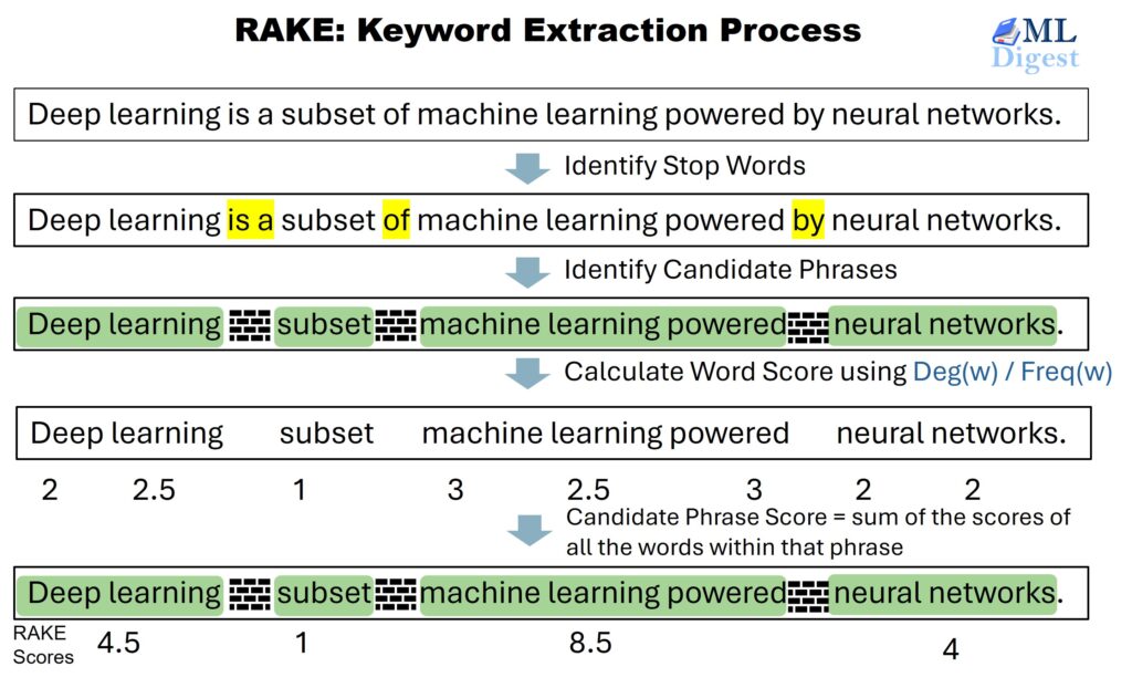
Take the sentence: “Deep learning is a subset of machine learning powered by neural networks.” After removing the stopwords (is, a, of, by), break the sentence at each stopword. The candidate phrases are “Deep learning”, “subset”, “machine learning powered”, and “neural networks”. - Compute Word Frequency:
For each word \(w\) in the candidate phrases, count how many times \(w\) appears across all phrases. This is the word’s frequency, \(freq(w)\). - Compute Word Degree:
For each word \(w\), sum the lengths of all phrases in which \(w\) appears. This is the word’s degree, \(deg(w)\).
$$ deg(w) = \sum_{p \in P,\; w \in p} len(p) $$
This step captures how often a word co-occurs with other words in multi-word phrases. - Calculate Word Scores:
For each word, compute the score as the ratio of degree to frequency:
$$ Score(w) = \frac{deg(w)}{freq(w)} $$- If a word always appears alone (for example, “subset”), \(deg = freq\), so the score is 1.
- If a word appears in longer phrases (for example, “learning” in “machine learning” and “deep learning”), its degree is higher relative to its frequency, boosting its score.
- Score Candidate Phrases:
For each candidate phrase \(p\), sum the scores of its constituent words:
$$ Score(p) = \sum_{w \in p} Score(w) $$
Longer, informative phrases tend to get higher scores if they are built from words with high degree-to-frequency ratios.
By following these steps, RAKE efficiently extracts and ranks keyword phrases, favoring those that are both frequent and well-connected within the text.
Where RAKE works well:
- Clean, grammatically correct text where stopwords behave predictably.
- You want interpretable phrase scores based on simple statistics.
- You have a good stopword list for the target language.
Where RAKE struggles:
- Highly noisy, non-standard text (for example, social media, code-mixed text).
- Domains where function words are not well captured by generic stopword lists.
- Very short documents, where computing meaningful degrees is harder.
Python Implementation
We can implement RAKE easily using the rake-nltk library.
!pip install rake_nltk
import nltk
nltk.download('stopwords')
nltk.download('punkt_tab')

from rake_nltk import Rake

# Initialize RAKE
# It uses the NLTK stopword list by default
r = Rake()

# Deep learning is a subset of machine learning that utilizes neural networks

# Our sample text
text = """Deep learning is a subset of machine learning powered by neural networks."""

# Extract keywords
r.extract_keywords_from_text(text)

# Get the ranked phrases with scores
# RAKE returns a list of tuples (score, phrase)
ranked_phrases = r.get_ranked_phrases_with_scores()

print("RAKE Scores:")
for score, phrase in ranked_phrases:
    print(f"{score:.2f}: {phrase}")
# Output RAKE Scores:
# 8.50: machine learning powered
# 4.50: deep learning
# 4.00: neural networks
# 1.00: subsetOutput Analysis (step-by-step):
To truly understand these numbers, it is helpful to look at the implicit co-occurrence structure. RAKE assumes that words appearing together in a phrase are related. The score is not just about how often a word appears (frequency), but how long the phrases are in which it appears (degree).
Here is the step-by-step calculation for the input: “Deep learning is a subset of machine learning powered by neural networks.”
Words: deep, learning, subset, machine, powered, neural, networks
(Note: “is”, “a”, “of”, “by” are treated as stopwords and removed)
Candidate Phrases:
- P1 = [deep, learning]
- P2 = [subset]
- P3 = [machine, learning, powered]
- P4 = [neural, networks]
Frequency (F):
- F(deep) = 1
- F(learning) = 2
- F(subset) = 1
- F(machine) = 1
- F(powered) = 1
- F(neural) = 1
- F(networks) = 1
Degree (D):
The degree of a word is the sum of the lengths of the phrases in which it appears.
- D(deep): Only in P1 (length 2). So, D(deep) = 2.
- D(learning): In P1 (length 2) and P3 (length 3). So, D(learning) = 2 + 3 = 5.
- D(machine): Only in P3 (length 3). So, D(machine) = 3.
- D(powered): Only in P3 (length 3). So, D(powered) = 3.
- D(neural): Only in P4 (length 2). So, D(neural) = 2.
- D(networks): Only in P4 (length 2). So, D(networks) = 2.
- D(subset): Only in P2 (length 1). So, D(subset) = 1.
Word Scores (S = D / F):
- WordScore(deep) = 2 / 1 = 2.0
- WordScore(learning) = 5 / 2 = 2.5
- WordScore(machine) = 3 / 1 = 3.0
- WordScore(powered) = 3 / 1 = 3.0
- WordScore(neural) = 2 / 1 = 2.0
- WordScore(networks) = 2 / 1 = 2.0
- WordScore(subset) = 1 / 1 = 1.0
Phrase Scores (Sum of Word Scores):
- machine learning powered:
WordScore(machine) + WordScore(learning) + WordScore(powered) =
\(3.0 + 2.5 + 3.0 = \mathbf{8.5}\) - deep learning:
WordScore(deep) + WordScore(learning)
\(2.0 + 2.5 = \mathbf{4.5}\) - neural networks:
WordScore(neural) + WordScore(networks)
\(2.0 + 2.0 = \mathbf{4.0}\) - subset:
WordScore(subset)
\(\mathbf{1.0}\)
This calculation reveals why “machine learning powered” ranks highest: it contains “learning” (a high-frequency bridge word across multiple phrases) and two other words that appear in a relatively long phrase, maximizing their individual degrees.
Part 2: YAKE (Yet Another Keyword Extractor)
Intuition: The “Statistical Detective”
While RAKE relies heavily on an external list of stopwords, YAKE is a “lone wolf.” It is an unsupervised, statistical method that does not depend on dictionaries or external corpora.
Imagine a detective looking at a document in a language they do not fully speak. How do they find the important words? They look for clues:
- Is the word capitalized? (Casing)
- Is it in the title or beginning? (Position)
- Does it appear often? (Frequency)
- Does it appear in different contexts? (Dispersion)
YAKE calculates a set of features for each word to determine its “uniqueness” and importance. Unlike many algorithms where a high score is good, in YAKE, the lower the score, the more important the keyword.
The Mechanics: The 5 Features
YAKE evaluates each word \(w\) based on five component scores. Let’s break down the intuition and the math for each.
1. Casing (\(T_{Case}\)): The “Formal Wear” Clue
Words that are capitalized (and are not just at the start of a sentence) are often Named Entities (like “NASA” or “Python”) or important concepts. YAKE gives a “bonus” (lower score) to words that frequently appear capitalized or as acronyms.
$$ T_{Case} = \frac{\max(TF(U), TF(A))}{ \ln(TF(w)) } $$
- Where \(TF(U)\) is the frequency of the word starting with an Uppercase letter.
- \(TF(A)\) is the frequency of the word as an Acronym.
2. Word Position (\(T_{Pos}\)): The “First Impression” Clue
In most documents, the main topic is introduced early—often in the title or the first paragraph. Words that appear at the beginning of the document are penalized less (get a better score) than those that only show up at the end.
$$ T_{Pos} = \ln(\ln(Median(Positions) + 1) + 1) $$
- This function grows slowly, but words concentrated at the start (low median position) get a significantly lower (better) score.
3. Word Frequency (\(T_{Freq}\)): The “Goldilocks” Clue
Frequency is a double-edged sword.
- Too Rare: Probably a typo or irrelevant detail.
- Too Frequent: Probably a stopword (like “the”, “and”).
- Just Right: The Keywords.
YAKE normalizes a word’s frequency against the mean and standard deviation of all word frequencies in the document to find this balance.
- The formula (simplified) penalizes words that are statistically “too frequent” (stopwords) while rewarding those that are frequent enough to be significant.
- \(T_{Freq} = \frac{Freq(w)}{\mu + \sigma}\) (Conceptual approximation)
4. Context Relatedness (\(T_{Rel}\)): The “Social Network” Clue
This is YAKE’s most clever feature. It measures the diversity of the words that appear to the left and right of our candidate.
- Stopwords are “Social Butterflies”: They appear next to everything. “The” appears next to “apple”, “car”, “sky”, “idea”. It has low relatedness (high diversity).
- Keywords are “Clique-y”: They appear in specific contexts. “Neural” appears next to “networks”, “processing”, “artificial”. It has high relatedness (low diversity).
$$ T_{Rel} = 1 + (DL + DR) \cdot \frac{Freq(w)}{MaxFreq} $$
- Where \(DL\) and \(DR\) count the number of different unique words to the left and right. A higher number of different neighbors increases this score (which is bad for the final ranking).
5. Sentence Spread (\(T_{Sentence}\)): The “Ubiquity” Clue
A word that appears in many different sentences is likely more significant than one that is repeated five times in a single sentence and never mentioned again.
$$ T_{Sentence} = \frac{SF(w)}{\#Sentences} $$
- Where \(SF(w)\) is the number of sentences in which \(w\) appears.
The Final Score (\(SF(w)\))
These five components are combined into a single score for each word. The goal is to find words that have the characteristics of a keyword (Capitalized, Early, Frequent-but-not-too-frequent, Specific Context) and combine them.
The Aggregation:
$$ S(w) = \frac{T_{Rel} \cdot T_{Pos}}{T_{Case} + \frac{T_{Freq}}{T_{Rel}} + \frac{T_{Sentence}}{T_{Rel}}} $$
How to read this equation:
- Numerator (\(T_{Rel} \cdot T_{Pos}\)): We want this to be small. We want words that appear early (small \(T_{Pos}\)) and have specific contexts (small \(T_{Rel}\) implies specific neighbors).
- Denominator: We want this to be large. We want words that are capitalized (\(T_{Case}\) contributes) and frequent (\(T_{Freq}\) contributes).
Finally, candidate phrases (n-grams) are scored by aggregating the scores of their member words. Remember: The lower the final score, the more important the keyword.
Where YAKE works well:
- Zero-Shot Extraction: Works on any language without setup.
- Noisy Text: Robust against informal text or web scrapes where grammar is shaky.
- Longer Documents: The statistical features (dispersion, relatedness) become more accurate as the text length increases.
Where YAKE struggles:
- Short Tweets/Titles: Statistics like “sentence spread” or “relatedness” are meaningless if the text is only 10 words long.
- Fixed Vocabularies: If you only want keywords from a specific list (e.g., medical codes), a statistical approach might “invent” new keywords you don’t want.
Python Implementation
!pip install yake

import yake

text = """Deep learning is a subset of machine learning powered by neural networks."""

# Initialize YAKE extractor
# lan: Language
# n: Max ngram size (phrase length)
# dedupLim: Deduplication threshold (to avoid similar phrases)
# top: Number of keywords to return
kw_extractor = yake.KeywordExtractor(lan="en", n=2, dedupLim=0.9, top=5)

keywords = kw_extractor.extract_keywords(text)

print("YAKE Scores (lower is better):")
for kw, score in keywords:
    print(f"{score:.4f}: {kw}")
# Output:
# YAKE Scores (lower is better):
# 0.0211: neural networks
# 0.0308: Deep learning
# 0.0514: machine learning
# 0.0514: learning powered
# 0.1125: DeepYou will typically see phrases such as “neural networks” and “Deep learning” ranked highly with low scores. Unlike RAKE, the absolute value of the score is less interpretable; what matters is the ranking of candidates.
Comparison and Best Practices
Now that we understand the engines under the hood, how do we choose between them?
| Feature | RAKE | YAKE |
|---|---|---|
| Dependency | Requires a Stopword List | Independent (Statistical) |
| Language Support | Good (if stoplist exists) | Excellent (Language Agnostic) |
| Speed | Very Fast | Fast |
| Single Documents | Good | Excellent |
| Corpus Required? | No | No |
When to use RAKE:
- Speed is critical: RAKE is computationally very lightweight.
- Standard Language: You are working with standard English (or a language with a good stoplist) and standard grammar.
- Short Texts: It works reasonably well on shorter snippets where statistical properties might not fully converge.
When to use YAKE:
- Multilingual/Unknown Language: You do not have a reliable stopword list.
- Noisy Text: YAKE’s statistical features (like casing and position) make it robust against informal text or web scrapes.
- Longer Documents: The statistical features (dispersion, relatedness) become more accurate with more text.
Practical Tips for Implementation
- Preprocessing Matters: Even though YAKE is robust, basic cleaning (removing HTML tags, fixing encoding errors) will always improve results.
- Tuning N-grams:
- Set
n=1if you only want single tags (e.g., for a tag cloud). - Set
n=2orn=3for keyphrases (e.g., “Machine Learning”, “Natural Language Processing”).
- Set
- Deduplication: Both libraries offer deduplication. Use it to avoid getting “Machine Learning” and “Learning” as two separate top keywords.
- Domain specifics: If you are working in a specific domain (for example, medical), RAKE allows you to add custom stopwords (like “patient”, “study”, “result”) to refine the extraction, whereas YAKE might need more text to “learn” that these are common background words.
- Combining RAKE and YAKE: In practice, combining both can work well:
- Use RAKE to propose high-recall candidate phrases.
- Use YAKE to re-rank or filter these candidates for higher precision.
- Using extracted keywords downstream:
- As features in classical ML models (for example, indicator features or TF–IDF over extracted phrases).
- As human-readable tags in dashboards and search interfaces.
- As input to LLM prompts (for example, “Summarize this document focusing on: [top keywords]”).
Conclusion
Keyword extraction is the bridge between human-readable content and machine-understandable data. RAKE builds this bridge by removing the noise (stopwords) and analyzing the structure of what remains. YAKE acts as an investigator, profiling words based on their behavior, position, and formatting.
By mastering these two algorithms, you equip yourself with lightweight, interpretable tools to summarize, categorize, and navigate the ocean of text data that defines modern machine learning workflows. They are often strong baselines and excellent companions to more advanced neural approaches.

Happy is a seasoned ML professional with over 15 years of experience. His expertise spans various domains, including Computer Vision, Natural Language Processing (NLP), and Time Series analysis. He holds a PhD in Machine Learning from IIT Kharagpur and has furthered his research with postdoctoral experience at INRIA-Sophia Antipolis, France. Happy has a proven track record of delivering impactful ML solutions to clients.
Subscribe to our newsletter!
