Post-Training Quantization Explained: How to Make Deep Learning Models Faster and Smaller

Large deep learning models are powerful but often too bulky and slow for real-world deployment. Their size, computational demands, and energy consumption make them impractical for mobile devices, IoT hardware, and other resource-limited environments. This gap between capability and usability is what model optimization aims to bridge.

To solve this, we turn to model optimization, a set of techniques designed to make models smaller, faster, and more efficient without sacrificing too much of their predictive power. One of the most effective optimization techniques is quantization.

There are two primary approaches to quantization:

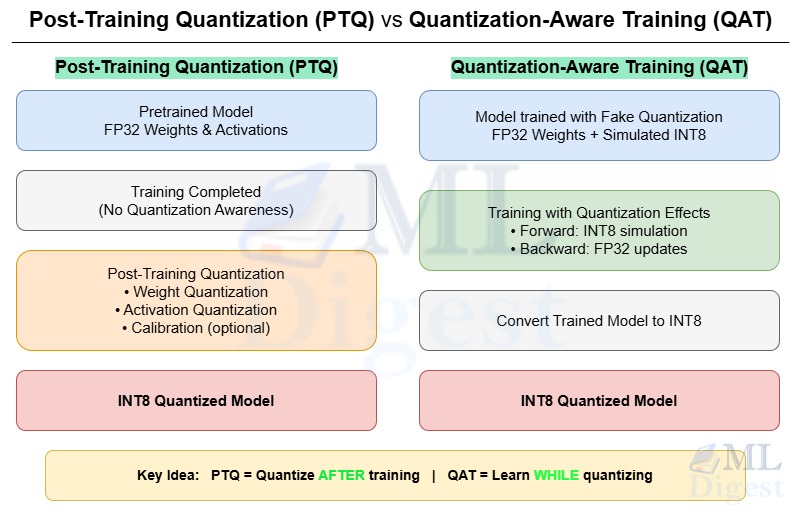
1. Quantization-Aware Training (QAT): This method simulates the effects of quantization during the training process. The model learns to adapt to the lower-precision format, which often results in higher accuracy. However, it requires a full retraining cycle and access to the original training dataset.
2. Post-Training Quantization (PTQ): This method converts a model to a lower-precision format after it has already been trained. It is a much simpler and faster process that does not require retraining.

This article will take a deep dive into the world of Post-Training Quantization, exploring how this powerful technique acts as an “easy button” for making deep learning models ready for the real world.

Quantization core idea: Scale and Zero-Point

At its heart, quantization is the process of reducing the number of bits used to represent a number. In deep learning, this typically means converting model parameters (weights) and activations from a high-precision 32-bit floating-point format (FP32) to a lower-precision format, most commonly an 8-bit integer format (INT8).

The magic behind quantization lies in a simple linear transformation. To map a floating-point value \(x\) to its quantized integer counterpart \(x_q\), we use two key parameters: a scale factor (s) and a zero-point (z).

The formula is:
$$ x_q = \text{round}\left(\frac{x}{s}\right) + z $$

And to de-quantize it back to a floating-point value:
$$ x = s \cdot (x_q – z) $$

• Scale (s): A positive floating-point number that defines the step size of the quantization. It determines how large a range of real values is mapped to a single integer value.
• Zero-Point (z): An integer that ensures the real value 0.0 is perfectly represented by a quantized integer. This is crucial for operations like padding with zeros.

We can visualize this mapping. Imagine we want to quantize FP32 values in the range [-10.0, 10.0] to INT8, which can represent integers from 0 to 255. The scale and zero-point would be calculated to map -10.0 to 0 and 10.0 to 255.

[Asymmetric vs Symmetric] and [Per-Channel vs Per-Tensor] Quantization

Deriving Scale and Zero-Point (Asymmetric Case)

Let \(x_{\min}\) and \(x_{\max}\) be the clipping range for a tensor, and let \(q_{\min}, q_{\max}\) be the integer range (for unsigned INT8: \(q_{\min}=0, q_{\max}=255\)). We want:
$$ x_{\min} \mapsto q_{\min}, \quad x_{\max} \mapsto q_{\max} $$
The scale is:
$$ s = \frac{x_{\max} – x_{\min}}{q_{\max} – q_{\min}} $$
The zero-point is chosen so that \(x=0\) maps exactly (if possible) to an integer:
$$ z = \text{round}\left(q_{\min} – \frac{x_{\min}}{s}\right) $$
The forward quantization then uses the previously stated affine relationship. If \(z\) falls outside \([q_{\min}, q_{\max}]\), the clipping range must be adjusted.

Symmetric Quantization

For symmetric quantization we select a range \([-R, R]\) (often \(R = \max(|x_{\min}|, |x_{\max}|)\)) and use a signed integer range (e.g., INT8: \([-127, 127]\)). Zero-point is fixed at zero. Scale becomes:
$$ s = \frac{R}{127} $$
Symmetric quantization simplifies kernels (no explicit zero-point) and can improve runtime efficiency. However, if the distribution of values is highly shifted away from zero, asymmetric mapping preserves representational fidelity by aligning zero precisely.

Numeric Example

Suppose activations after calibration are clipped to \([-2.4, 3.6]\). For unsigned INT8 (\([0, 255]\)):
$$ s = \frac{3.6 – (-2.4)}{255 – 0} = \frac{6.0}{255} \approx 0.02353 $$
$$ z = \text{round}\left(0 – \frac{-2.4}{0.02353}\right) = \text{round}(102.0) = 102 $$
Quantizing \(x = 1.0\):
$$ x_q = \text{round}\left(\frac{1.0}{0.02353}\right) + 102 = \text{round}(42.5) + 102 = 145 $$
De-quantizing:
$$ \hat{x} = 0.02353 \cdot (145 – 102) = 0.02353 \cdot 43 \approx 1.012 $$
The small discrepancy (\(\approx 0.012\)) is the quantization error.

Quantization Error and MSE Approximation

Assuming a value is uniformly distributed inside a quantization bin of width \(\Delta = s\), the mean squared quantization error for uniform quantization is approximately:
$$ \text{MSE} \approx \frac{\Delta^2}{12} $$
This provides intuition: reducing $s$ (finer granularity) reduces error, but requires a larger integer range or higher bit width.

Rounding Considerations

Standard implementations use nearest integer rounding. Stochastic rounding (rare in standard deployment) can reduce bias accumulation for ultra-low bit widths (INT2/INT4) by randomly rounding up or down proportionally to the fractional part.

Per-Channel vs Per-Tensor

For weight tensors (e.g., convolutional filters), distributions vary significantly across output channels. Assigning each channel its own scale (and sometimes zero-point) reduces error, especially for layers with heterogeneous magnitude patterns. Activations are commonly quantized per-tensor to limit runtime metadata overhead.

Trade-Off Summary

• Asymmetric: Better when data range is shifted; requires storing zero-point.
• Symmetric: Simplifies arithmetic (often faster); may incur extra error if distribution mean is far from zero.
• Per-channel: Improved accuracy for weights; modest metadata increase.
• Per-tensor: Lower overhead; possible accuracy loss for heterogeneous distributions.

Post-Training Quantization (PTQ): The “Easy Button” for Optimization

Now, let us focus on PTQ. As the name suggests, PTQ is applied to a model that has already been trained. It is a lightweight, fast, and convenient optimization method.

Think of it like taking a finished, high-resolution digital photograph (our FP32 model) and compressing it into a JPEG (our INT8 model) to easily share it online. You are not retaking the photo or changing its content; you are just making it smaller and more portable.

The primary advantages of PTQ are:

• Simplicity: It is far less complex than QAT. You do not need to modify the training code or set up a complex training pipeline.
• Speed: The process is extremely fast, often taking only a few minutes, whereas QAT can take hours or days of retraining.
• No Original Data Needed: You do not need the original, massive training dataset. PTQ works with a small, representative “calibration dataset,” which can be as small as a few hundred samples.

How PTQ Works: The Calibration Process

The central challenge in PTQ is determining the right scale and zero-point for the weights and, more importantly, the activations. The distribution of weights is fixed after training, so we can easily calculate their quantization parameters. However, the distribution of activations (the outputs of each layer) is input-dependent and can vary wildly.

PTQ is best understood with the following steps:

1. Weights Quantization:
   The first step involves quantizing the model weights (and biases), which are fixed after training. This happens offline (before inference) as they are static parameters. Typically, per-channel quantization is used to minimize quantization error, as each channel in a layer may have a different value distribution.
2. Activations Quantization (Calibration):
   The next step is calibrating the activations by running a representative dataset through the full-precision model. During this process, statistics (like min/max values or histogram distributions) of the activations are collected for each layer, allowing for the determination of optimal scale and zero-point values for each layer’s activations. This is a dynamic (during inference) process that adapts to the input data. Calibration ensures that the quantized model maintains as much accuracy as possible during inference, despite the reduced precision.
3. Final Conversion/Inference:
   The final quantized model (with quantized weights and the derived parameters for activations) is then used for inference, where both weights and activations are quantized to low-precision types (e.g., INT8) for the actual computation.

This multi-step approach is essential for achieving reliable performance in PTQ, as it balances the static nature of weights with the dynamic, data-dependent behavior of activations.

Calibration is the process of feeding a small, representative set of data through the model and observing the distribution of activations at each layer. This allows the quantization tool to determine the optimal clipping range [min, max] for the activations at each layer, which is then used to calculate the scale and zero-point.

There are several methods for choosing this clipping range during calibration:

1. Min-Max Quantization: This is the simplest method. The tool records the absolute minimum and maximum activation values seen during calibration and uses them as the clipping range. While easy, this method is very sensitive to outliers. A single extreme value can ruin the quantization for all other values.
2. Mean-Square Error (MSE) Quantization: This method is more robust. It searches for a clipping range that minimizes the mean squared error between the original floating-point activations and the quantized activations. This often leads to better accuracy than simple min-max.
3. Entropy (KL-Divergence) Quantization: This is a more advanced and often most effective technique. It treats the distribution of activations as a probability distribution and searches for a clipping range that minimizes the KL-Divergence between the original FP32 distribution and the quantized INT8 distribution. In essence, it tries to preserve the most information possible during the conversion, leading to higher accuracy.

The PTQ Workflow in Practice

Applying PTQ using modern deep learning frameworks is a straightforward process:

1. Start with a Pre-trained FP32 Model: You begin with your fully trained, high-precision model.
2. Prepare a Calibration Dataset: Select a small (e.g., 100-500 samples) but representative subset of your validation or training data. This data should reflect the real-world data the model will see in production.
3. Choose a PTQ Tool: Use a library like PyTorch’s quantization module or TensorFlow Lite’s converter.
4. Weights Quantization: The model’s weights (and biases) are analyzed and quantized offline (before inference) as they are static parameters.
5. Run Calibration: The tool will run a forward pass of the model on the calibration dataset. During this pass, it will insert “observers” at each layer to record the distribution (like min/max values or histograms) of activations.
6. Calculate Quantization Parameters: Based on the observed distributions, the tool calculates the optimal scale and zero-point for each layer’s activations using one of the methods described above (e.g., KL-Divergence).
7. Convert the Model: The tool converts the model’s weights to INT8 and stores the calculated activation quantization parameters. The model is now ready for low-precision inference.
8. Deploy the INT8 Model: The resulting model is smaller, faster, and ready for deployment on resource-constrained devices.

Challenges and Advanced Techniques

While PTQ is powerful, it is not a silver bullet. The most common issue is a drop in accuracy. This happens because the quantization process—rounding values and clipping outliers—is inherently lossy.

To combat this, several advanced techniques have been developed:

• Weight-Only Quantization: Only the weights are quantized (e.g., to INT8 or INT4) and stored in low precision. The activations remain in a higher precision format like FP32 or FP16 during inference, but operations are often performed in INT8 for speed.
• Full Integer Quantization (Weights + Activations): Both the weights and the activations are quantized, typically to INT8, enabling maximum performance gains on hardware optimized for integer arithmetic. This variant requires the calibration step to determine the activation quantization parameters.
• Per-Channel Quantization: Instead of using a single scale and zero-point for an entire weight tensor (per-tensor), this technique uses different parameters for each output channel of a convolutional filter. This provides a more fine-grained and accurate quantization, especially for layers with widely varying weight distributions across channels.
• Bias Correction: Quantization can introduce a slight bias, causing the mean of a layer’s output to shift. Bias correction is a post-calibration step that adjusts the bias term of a quantized layer to counteract this shift, helping to recover lost accuracy.
  For a layer producing floating outputs \(y_{fp}\) and quantized outputs \(y_{int}\) with means \(\mu_{fp}, \mu_{int}\):
  $$ b_{new} = b_{old} + (\mu_{fp} – \mu_{int}) $$
• Mixed-Precision Quantization: Some layers in a network are more sensitive to quantization than others. If a model’s accuracy drops too much after full INT8 quantization, you can use a mixed-precision approach. This involves strategically keeping a few sensitive layers in a higher precision (like FP16 or even FP32) while quantizing the rest. This provides a trade-off, improving accuracy while still retaining most of the performance benefits.

Decision Checklist (PTQ Suitability)

Use PTQ when most boxes below can be checked:

• Model is already fully trained; retraining budget is limited.
• Representative calibration data (≥ 100 samples) is available.
• Target hardware accelerates INT8 (FBGEMM, QNNPACK, TensorRT, NNAPI, OpenVINO).
• Acceptable accuracy drop threshold defined (e.g., ≤ 1% top-1).
• Latency or memory is a deployment bottleneck.
• Regulatory or safety constraints do not mandate retraining with QAT.
• Layer sensitivity profile does not show extreme fragility requiring full QAT.

Calibration Dataset Design and Pitfalls

Calibration quality often determines PTQ success. A poorly chosen calibration set yields distorted activation statistics, leading to aggressive clipping or overly wide ranges. Below are guidelines.

• Representativeness:
  • Select calibration samples that closely match the data distribution expected in production.
  • For image tasks, include a range of classes, lighting conditions, and resolutions.
  • For language models, use a mix of formal, informal, and domain-specific text.
• Sample Size:
  • Use 100–500 samples for vision models; deeper transformers may require 512–2048 sequences for stable LayerNorm statistics.
  • Monitor running min/max values to determine when distributions stabilize and additional samples yield diminishing returns.
• Diversity vs Noise:
  • Avoid calibration sets dominated by edge cases, which can inflate activation ranges and increase quantization error.
  • Do not use overly narrow sets, as they may under-represent distribution tails and cause clipping in deployment.
  • Prefer stratified sampling to balance diversity and representativeness.
• Preprocessing Consistency:
  • Ensure calibration data undergoes the same preprocessing steps (e.g., normalization, resizing, tokenization) as inference data.
  • Inconsistent preprocessing can shift activation distributions and degrade quantization quality.
• Outlier Handling:
  • Address rare, large-magnitude activations by:
    • Applying clipping heuristics (MSE or KL-based selection often mitigates outliers automatically).
    • Using smoothing transformations (e.g., activation scaling as in SmoothQuant).
    • Employing mixed precision for layers sensitive to outliers.
• Monitoring:
  • Log per-layer min/max histograms during calibration.
  • Identify unstable layers with expanding ranges and consider increasing sample count or isolating them for mixed precision treatment.
• Reuse vs Fresh Capture:
  • Periodically recalibrate if production data distribution shifts over time.
  • Regular recalibration helps maintain accuracy as data evolves.

Practical Checklist

1. 100–500 representative samples collected.
2. Preprocessing identical to deployment.
3. Layer-wise activation ranges logged and stabilized.
4. Outliers assessed (decide clip strategy or smoothing).
5. Sensitivity list drafted (layers earmarked for fallback).

Calibration is not an afterthought; it is the empirical foundation upon which reliable quantization parameters rest.

Conclusion: When to Choose PTQ

Post-Training Quantization is an indispensable tool in the modern MLOps toolkit. It provides a simple, fast, and effective way to optimize deep learning models for real-world deployment.

You should consider using PTQ when:

• You need to deploy a model on resource-constrained hardware (edge devices, mobile phones).
• The original training pipeline or dataset is not available.
• Development time is limited, and you need a quick optimization solution.
• A small to moderate drop in accuracy is an acceptable trade-off for significant gains in performance and efficiency.

By transforming heavy, powerful models into lightweight, nimble performers, PTQ makes state-of-the-art deep learning more accessible and practical than ever before, paving the way for its integration into countless everyday applications.

FAQ

What are the Large Language Model (LLM) Specific PTQ Techniques?

Quantizing large transformer models introduces distinct challenges: wide activation dynamic ranges (especially post LayerNorm), sensitivity of attention mechanisms, and memory bandwidth constraints dominating latency.

LLM.int8(): Selective retention of outlier channels in higher precision while quantizing the bulk of matrix multiplication pathways to INT8. Outliers (e.g., channels with much larger magnitudes) are detected and processed separately, mitigating severe accuracy drops.

SmoothQuant: Balances activation and weight magnitudes by scaling activations down and weights up multiplicatively prior to quantization. Given an activation tensor $A$ and weight $W$, apply scaling factors $\alpha$ so that outlier activation values are suppressed, reducing range explosion. After transformation, standard INT8 quantization yields smaller error. SmoothQuant is especially effective for feed-forward and attention projection layers.

GPTQ (Post-Training, Second-Order Optimization):
GPTQ performs layer-wise quantization using a Hessian-based approximation to model and compensate for quantization error. Weights are quantized sequentially, with each step adjusting for the error introduced in previous steps. This approach achieves near-original perplexity, even at 4-bit precision, for many large language models. While computationally intensive, GPTQ does not require retraining.

AWQ (Activation-Aware Weight Quantization):
AWQ prioritizes the preservation of critical activation pathways during quantization. By identifying channels that are most influential to output activations, AWQ applies tailored scaling to minimize quantization error in these regions. This targeted approach helps maintain model accuracy, especially in layers where certain channels dominate the output.

Weight-Only 4-Bit Quantization:
This technique stores model weights in INT4 format while keeping activations in higher precision (FP16 or BF16). The memory savings are substantial for models with billions of parameters. During inference, weights are dequantized on the fly for matrix multiplication, while activation quantization is often deferred or omitted to preserve softmax stability.

LayerNorm and Softmax Considerations:
LayerNorm outputs typically have narrow distributions, but small shifts can significantly affect downstream attention mechanisms. These layers are often kept in FP16 or quantized with higher bit widths (such as 8-bit symmetric quantization). Softmax inputs, which are highly sensitive to quantization, are usually left in higher precision to avoid destabilizing probability distributions.

Practical LLM Quantization Strategy:

1. Profile magnitude distributions for weights and activations in each layer.
2. Apply SmoothQuant pre-scaling to balance activation and weight ranges.
3. Quantize primary linear layers using weight-only 4-bit methods (GPTQ or AWQ).
4. Retain embedding layers, LayerNorm, and logits head in FP16.
5. Validate model performance using perplexity and downstream task metrics.
6. Refine outlier handling, employing LLM.int8 fallback for layers with excessive quantization error.

Mixed Precision Note:
A hybrid approach—combining weight-only 4-bit quantization with FP16 activations and selective INT8 quantization for feed-forward layers—can optimize both memory usage and accuracy. Benchmarking cross-layer latency is essential, as dequantization overhead may offset theoretical gains if kernel implementations are not fully optimized.

LLM-oriented quantization extends standard PTQ concepts with targeted treatments for distribution outliers and memory-bound execution patterns.

What are the main challenges when applying PTQ to large language models (LLMs)?

The main challenges when applying PTQ to LLMs include handling the wide dynamic range of activations, especially after LayerNorm layers, which can lead to significant quantization errors. Additionally, attention mechanisms are particularly sensitive to quantization, and improper handling can degrade model performance. Memory bandwidth limitations also play a crucial role, as LLMs are often memory-bound during inference. Techniques like SmoothQuant, LLM.int8(), and weight-only 4-bit quantization have been developed to address these challenges effectively.

How can PTQ be adapted for different model architectures?

PTQ can be adapted for different model architectures by considering the specific characteristics and requirements of each architecture. This may involve customizing the quantization strategy, such as using different bit widths for different layers, applying layer-specific calibration techniques, or leveraging architectural features like skip connections or attention mechanisms to improve quantization robustness. Additionally, incorporating domain knowledge about the model’s task and data can help inform more effective quantization approaches.

What are some common pitfalls to avoid when implementing PTQ?

Common pitfalls when implementing PTQ include using an unrepresentative calibration dataset, which can lead to poor activation range estimation and significant accuracy loss. Another pitfall is neglecting to monitor layer-wise activation distributions, which can help identify layers that may require special handling or mixed-precision treatment. Additionally, failing to account for outliers in activation values can result in excessive clipping and quantization error. Finally, not validating the quantized model’s performance on a relevant dataset can lead to unexpected drops in accuracy during deployment.

How does PTQ compare to Quantization-Aware Training (QAT) in terms of accuracy and deployment complexity?

PTQ is generally simpler and faster to implement than QAT, as it does not require retraining the model. However, QAT often achieves higher accuracy because the model learns to adapt to quantization effects during training. PTQ may result in a more significant drop in accuracy, especially for models with sensitive layers or wide activation distributions. In terms of deployment complexity, PTQ is less complex since it can be applied to pre-trained models without modifying the training pipeline. QAT requires a more involved setup but can yield better performance for applications where accuracy is critical.