Perplexity (PPL): what it measures, how to compute it, and when it misleads

Perplexity answers one narrow question:

When the true next token is revealed, how confused/uncertain is the model?

It is a likelihood-based metric for next-token prediction. It is invaluable for training curves and careful, apples-to-apples comparisons. It is also routinely misused as a proxy for generation quality.

What this note covers: intuition, math, evaluation gotchas, a toy example, and a practical reference implementation.

Intuition: the “effective number of choices”

Perplexity can be (roughly) understood as the model’s effective branching factor: how many next-token choices it behaves as if it has.

Given a prefix like “The sky is …”, a confused model might spread probability mass evenly across many words, while a smart model concentrates mass on plausible continuations (like “blue” or “overcast”).

• If a model has a perplexity of 10, it is as confused as if it were choosing uniformly from 10 possible next tokens at each step.
• An ideal model for a specific deterministic sentence would have a perplexity of 1 (it knows exactly what comes next).

A PPL of $k$ roughly means the model behaves as if it is choosing among $k$ equally likely options at each step.

Caveat: This intuition assumes uncertainty is spread somewhat uniformly. In practice, models are very confident on function words and far less confident on content words, so PPL is a blend of “easy” and “hard” positions.

What perplexity is (and is not)

What it is: Perplexity measures the uncertainty of a language model—how much probability mass a language model assigns to the observed text under next-token prediction. A high perplexity means the model finds it difficult to predict the next word in a sentence; it considers many different words as equally likely. A low perplexity means the model is very confident about its prediction for the next word, which aligns well with the actual text.

Why it matters:

• Model Comparison: Perplexity provides a standard benchmark to compare the performance of different language models. If Model A has a lower perplexity than Model B on the same dataset, Model A is generally considered better.
• Training Guide: During the training process, data scientists monitor the perplexity score. A decreasing perplexity over time is a strong indicator that the model is learning and improving.
• Distribution match (not “quality”): Low PPL usually correlates with better next-token prediction on that distribution, which can correlate with fluency. However, it is not a direct measure of helpfulness, factuality, reasoning, or preference-aligned generation.

What it is not:

• Not a direct measure of factuality, helpfulness, safety, or reasoning.
• Not a number you can compare across different tokenizers or different evaluation setups.

Perplexity is only comparable under identical tokenization and identical scoring protocol.

Visualizing Perplexity: Confidence vs. Confusion

Let us visualize the probability distributions that lead to low vs. high perplexity. Consider the context: “The cat sat on the _“.

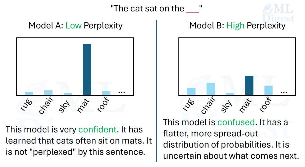
• Low-Perplexity Model: This model confidently predicts “mat” as the next word, assigning it a high probability (e.g., 0.9). The remaining words like “roof,” “chair,” and “rug” receive very low probabilities. This indicates that the model is well-trained and understands the context of the sentence.
• High-Perplexity Model: In contrast, this model is uncertain and assigns more even probabilities across several options: “mat” (0.3), “roof” (0.2), “chair” (0.25), and “rug” (0.15). This spread of probabilities indicates confusion, as the model does not have a clear understanding of what word fits best in the context.

The Math: From “Surprise” to a Single Number

We have established the intuition: we want a number that represents the “effective number of choices.” How do we calculate that from the model’s raw output?

Let us assume our model assigns probabilities to a sequence of $N$ tokens: $w_1, w_2, \dots, w_N$.

1. The Probability of the Sequence

First, we look at the probability the model assigns to the entire correct sequence. In a causal language model, this is the product of the conditional probabilities of each word:

$$
P(W) = \prod_{i=1}^{N} P(w_i \mid w_{<i})
$$

If the model is good, this number $P(W)$ will be high (close to 1). If the model is bad, it will be tiny (close to 0).

2. Cross-entropy / NLL (what the loss measures)

Because multiplying probabilities results in impossibly small numbers (underflow), we work in log space. We take the logarithm of the probabilities and maximize that (or minimize the negative).

Cross-entropy measures how different a model distribution $q$ is from a data distribution $p$:

$$\text{Cross-Entropy}(p, q) = – \sum_x p(x) \log_2 q(x)$$

If $p$ is a one-hot distribution over the observed next token, this becomes the negative log-probability of the observed token:

$$\text{Cross-Entropy}(p, q) = -\log_2 q(\text{correct word})$$

For an entire sequence of $N$ tokens, the average cross-entropy (base 2, in bits/token) is:

$$H_2 = – \frac{1}{N} \sum_{i=1}^{N} \log_2 P(w_i \mid w_{<i})$$

This formula calculates the average “surprise” the model feels at each word in the sentence.

In natural logarithm (base $e$), the average cross-entropy ($H$) is:

$$
H = -\frac{1}{N} \sum_{i=1}^{N} \ln P(w_i \mid w_{<i})
$$

• $H$ is the average “surprisal” per token.
• If we use base $e$, the unit of $H$ is nats/token.
• If we use base 2, the unit is bits/token.

Thus, training language models typically minimizes cross-entropy, which is the same as minimizing the average negative log-likelihood (NLL) of the observed next token under teacher forcing.

Connection back to intuition: when the model assigns a small probability to the true next token, $-\ln p$ becomes large. Averaging these penalties across tokens yields the loss; exponentiating that average yields perplexity.

3. Perplexity (the exponentiated loss)

Perplexity is the exponentiation of the cross-entropy. It brings us back from “log-space” to “probability-space” (and branching factors).

$$
\text{PPL} = \exp(H)
$$

If you used base 2 (bits), the relationship is:

$$
\text{PPL} = 2^{H_2}
$$

Why this matters: This explains the “effective branching factor” intuition. If your loss is 2 bits per token, your perplexity is $2^2 = 4$, meaning the model behaves (very roughly) like it is choosing among about 4 equally likely options per token.

Bits-per-token vs. Perplexity (Cheatsheet)

Researchers often report bits per token (BPT), i.e. $H_2$, because it is additive.

• Reducing loss from 4.1 to 4.0 bits is the same effort as reducing from 2.1 to 2.0 bits.
• However, in Perplexity space, the first is a drop of ~1.2 PPL, while the second is a drop of ~0.3 PPL.
• If $H$ is in nats/token, then $\text{BPT} = H/\ln 2$ and $\text{PPL} = e^H$.
• If $H_2$ is in bits/token, then $\text{PPL} = 2^{H_2}$.

Conversion Table (Approximation):

To convert manually:

1. Loss to PPL: If your training loss is $3.0$ (nats), then $\text{PPL} = e^{3.0} \approx 20.08$.
2. PPL to Bits: If $\text{PPL} = 20.08$, then $\text{Bits per Token} = \log_2(20.08) \approx 4.33$.
3. Additive vs. Multiplicative: A simpler way to reason about improvement is using bits. A reduction of 0.1 bits/token is significant, regardless of the baseline perplexity.

Critical Evaluation “Gotchas”

Perplexity is notoriously sensitive. If you see a paper reporting a PPL of 12.0 and another reporting 14.0, you cannot say the first is better unless they used the exact same protocol.

1. The Tokenizer Trap:
   • Scenario: Model A uses a huge vocabulary (100k words). Model B uses a small one (30k words).
   • Result: Model A might have a higher perplexity per token, but is actually more efficient because it produces fewer tokens overall (higher information density per token).
   • Fix: Only compare PPL between models sharing the same tokenizer.
2. Context Length & Stride:
   • Scenario: You evaluate a long document. Do you reset the model’s memory after every 2048 tokens? Or do you slide a window safely?
   • Result: Resetting memory causes massive spikes in loss at the start of every chunk (context blindness).
   • Fix: Use a Sliding Window evaluation (code below).
3. BOS/EOS Token Handling:
   • Scenario: Some libraries insert a BOS (Beginning of Sequence) token.
   • Result: The first token is trivial to predict (it is always the start). If you include this “free win” in your average, your PPL drops artificially.
   • Fix: Define clearly if you are skipping the first token. Score only next-token predictions over normal text tokens; do not score any artificially inserted BOS toke.
4. Normalization (Word vs. Token):
   • Scenario: Some older papers normalize by word count, not token count.
   • Result: PPL numbers are completely incompatible.
   • Fix: Standard for LLMs is per-token.

Worked toy example (why it is a geometric mean)

Suppose a model assigns probabilities to the correct next token across 4 steps: $[0.5, 0.25, 0.25, 0.5]$.

• Average NLL in nats: $H = -\frac{1}{4}(\ln 0.5 + \ln 0.25 + \ln 0.25 + \ln 0.5)$
• PPL: $\exp(H) = (0.5\cdot 0.25\cdot 0.25\cdot 0.5)^{-1/4}$

So PPL is the inverse geometric mean of the assigned probabilities.

Comparison Template (Copy to Experiment Log)

One more grown-up caveat: data leakage can dominate PPL. If your eval set overlaps with training data (common with web-scale corpora), reported PPL can be misleading as a measure of generalization.

When PPL is the right tool

• Training tracking: monitor likelihood as you train and tune.
• Apples-to-apples LM comparisons: same dataset + tokenizer + protocol.
• Regression tests: detect model or preprocessing changes that silently degrade next-token prediction.

Implementation: The Sliding Window Technique

We now have the formula and the intuition. How do we compute this for a long document (like a book) when our model has a fixed Context Window (e.g., 2048 tokens)?

The Problem with Discrete Chunks

If we simply chopped the text into non-overlapping chunks ([0:2048], [2048:4096]), the model would suffer at the boundaries. The word at position 2049 would see zero context, yielding a huge artificial loss.

The Solution: Sliding Windows

We treat the text as a stream. We move a window forward by a stride (e.g., 512 tokens).

• For each new window, we only calculate the loss on the new tokens (the stride).
• However, we provide the maximum possible history as context for those new tokens.

Python Implementation

This implementation handles the sliding window logic, ensuring every token (except the very first few) has full context.

import torch
import math
from tqdm import tqdm
from transformers import AutoModelForCausalLM, AutoTokenizer

def calculate_perplexity(
    model: AutoModelForCausalLM,
    tokenizer: AutoTokenizer,
    text: str,
    stride: int = 512,
    device: str = "cuda"
) -> float:
    """
    Computes perplexity on a long text using a sliding window strategy.

    Args:
        model: The causal language model.
        tokenizer: The corresponding tokenizer.
        text: The input text to evaluate.
        stride: Step size for the sliding window.
                Smaller stride = more overlap = better context = slower compute.
        device: 'cuda' or 'cpu'.

    Returns:
        dict: {'ppl': float, 'bits_per_token': float, 'tokens': int}
    """
    model.eval()

    # 1. Tokenize the entire text as one long sequence
    # Note: We do not truncate here; we handle chunks manually.
    encodings = tokenizer(text, return_tensors="pt", add_special_tokens=False)

    # max_length is the model's maximum context window.
    # Hugging Face model configs vary; prefer max_position_embeddings when present.
    max_len = getattr(model.config, "max_position_embeddings", None)
    if max_len is None:
        max_len = getattr(model.config, "n_positions", None)
    if max_len is None:
        raise ValueError("Could not infer model context length from config.")
    input_ids = encodings.input_ids.to(device)
    seq_len = input_ids.size(1)

    nlls = []
    total_scored_tokens = 0

    # 2. Iterate over the sequence with a sliding window
    # Protocol: feed a window of up to max_len tokens ending at end_loc,
    # and score only the last trg_len tokens (new tokens).
    prev_end_loc = 0
    for begin_loc in tqdm(range(0, seq_len, stride)):

        end_loc = min(begin_loc + max_len, seq_len)
        trg_len = end_loc - prev_end_loc

        # Prepare the input chunk
        # Note: We might grab context from *before* begin_loc if allowed,
        # but for a simple sliding window, we usually just process [begin_loc : end_loc]
        # and mask out the early parts if we wanted true "overlap".

        # More robust approach typically used in HuggingFace:
        # Input: [max(0, end_loc - max_len) : end_loc]
        # Target: Same as input
        # Mask: Everything EXCEPT the last 'stride' tokens.

        # Start of the window (can go back before 'begin_loc' to fill context)
        input_start = max(0, end_loc - max_len)

        input_ids_chunk = input_ids[:, input_start:end_loc]
        target_ids = input_ids_chunk.clone()

        # Mask out the context tokens. We only want to calculate loss for
        # the tokens that are new to this stride (the right-most part).
        # Mask out context tokens. Only score the last trg_len positions.
        target_ids[:, :-trg_len] = -100  # PyTorch ignore index

        with torch.no_grad():
            outputs = model(input_ids_chunk, labels=target_ids)

            # outputs.loss is mean NLL over unmasked labels.
            nlls.append(outputs.loss * trg_len)
            total_scored_tokens += trg_len

        prev_end_loc = end_loc
        if end_loc == seq_len:
            break

    # 3. Aggregate
    # Sum all NLLs and divide by total tokens processed
    total_nll = torch.stack(nlls).sum()
    if total_scored_tokens == 0:
        raise ValueError("No tokens were scored. Is the input text empty?")

    avg_nll = (total_nll / total_scored_tokens).item()
    ppl = float(math.exp(avg_nll))
    bpt = float(avg_nll / math.log(2))

    return {"ppl": ppl, "bits_per_token": bpt, "tokens": int(total_scored_tokens)}

# Example Usage
if __name__ == "__main__":
    model_id = "gpt2"
    tokenizer = AutoTokenizer.from_pretrained(model_id)

    # Determine device dynamically
    device = "cuda" if torch.cuda.is_available() else "cpu"
    print(f"Using device: {device}")

    model = AutoModelForCausalLM.from_pretrained(model_id).to(device)

    text = "Machine learning is a field of inquiry devoted to understanding and building methods that 'learn'..."

    result = calculate_perplexity(model, tokenizer, text, device=device)
    print(f"\n\nPerplexity: {result['ppl']:.2f}")
    print(f"Bits per Token: {result['bits_per_token']:.2f}")
# Expected Output:
#     Perplexity: 69.08
#     Bits per Token: 6.11

import torch
import math
from tqdm import tqdm
from transformers import AutoModelForCausalLM, AutoTokenizer

def calculate_perplexity(
    model: AutoModelForCausalLM,
    tokenizer: AutoTokenizer,
    text: str,
    stride: int = 512,
    device: str = "cuda"
) -> float:
    """
    Computes perplexity on a long text using a sliding window strategy.

    Args:
        model: The causal language model.
        tokenizer: The corresponding tokenizer.
        text: The input text to evaluate.
        stride: Step size for the sliding window.
                Smaller stride = more overlap = better context = slower compute.
        device: 'cuda' or 'cpu'.

    Returns:
        dict: {'ppl': float, 'bits_per_token': float, 'tokens': int}
    """
    model.eval()

    # 1. Tokenize the entire text as one long sequence
    # Note: We do not truncate here; we handle chunks manually.
    encodings = tokenizer(text, return_tensors="pt", add_special_tokens=False)

    # max_length is the model's maximum context window.
    # Hugging Face model configs vary; prefer max_position_embeddings when present.
    max_len = getattr(model.config, "max_position_embeddings", None)
    if max_len is None:
        max_len = getattr(model.config, "n_positions", None)
    if max_len is None:
        raise ValueError("Could not infer model context length from config.")
    input_ids = encodings.input_ids.to(device)
    seq_len = input_ids.size(1)

    nlls = []
    total_scored_tokens = 0

    # 2. Iterate over the sequence with a sliding window
    # Protocol: feed a window of up to max_len tokens ending at end_loc,
    # and score only the last trg_len tokens (new tokens).
    prev_end_loc = 0
    for begin_loc in tqdm(range(0, seq_len, stride)):

        end_loc = min(begin_loc + max_len, seq_len)
        trg_len = end_loc - prev_end_loc

        # Prepare the input chunk
        # Note: We might grab context from *before* begin_loc if allowed,
        # but for a simple sliding window, we usually just process [begin_loc : end_loc]
        # and mask out the early parts if we wanted true "overlap".

        # More robust approach typically used in HuggingFace:
        # Input: [max(0, end_loc - max_len) : end_loc]
        # Target: Same as input
        # Mask: Everything EXCEPT the last 'stride' tokens.

        # Start of the window (can go back before 'begin_loc' to fill context)
        input_start = max(0, end_loc - max_len)

        input_ids_chunk = input_ids[:, input_start:end_loc]
        target_ids = input_ids_chunk.clone()

        # Mask out the context tokens. We only want to calculate loss for
        # the tokens that are new to this stride (the right-most part).
        # Mask out context tokens. Only score the last trg_len positions.
        target_ids[:, :-trg_len] = -100  # PyTorch ignore index

        with torch.no_grad():
            outputs = model(input_ids_chunk, labels=target_ids)

            # outputs.loss is mean NLL over unmasked labels.
            nlls.append(outputs.loss * trg_len)
            total_scored_tokens += trg_len

        prev_end_loc = end_loc
        if end_loc == seq_len:
            break

    # 3. Aggregate
    # Sum all NLLs and divide by total tokens processed
    total_nll = torch.stack(nlls).sum()
    if total_scored_tokens == 0:
        raise ValueError("No tokens were scored. Is the input text empty?")

    avg_nll = (total_nll / total_scored_tokens).item()
    ppl = float(math.exp(avg_nll))
    bpt = float(avg_nll / math.log(2))

    return {"ppl": ppl, "bits_per_token": bpt, "tokens": int(total_scored_tokens)}

# Example Usage
if __name__ == "__main__":
    model_id = "gpt2"
    tokenizer = AutoTokenizer.from_pretrained(model_id)

    # Determine device dynamically
    device = "cuda" if torch.cuda.is_available() else "cpu"
    print(f"Using device: {device}")

    model = AutoModelForCausalLM.from_pretrained(model_id).to(device)

    text = "Machine learning is a field of inquiry devoted to understanding and building methods that 'learn'..."

    result = calculate_perplexity(model, tokenizer, text, device=device)
    print(f"\n\nPerplexity: {result['ppl']:.2f}")
    print(f"Bits per Token: {result['bits_per_token']:.2f}")
# Expected Output:
#     Perplexity: 69.08
#     Bits per Token: 6.11

Interpreting the Results

When you run the script, here is what the numbers mean:

• PPL ~1 – 10: The model is predicting simple, structured text (like simple code or repetitive logs).
• PPL ~10 – 20: Standard, fluent English text. The model is mildly surprised but generally accurate.
• PPL ~50 – 100: Highly complex, technical, or unfamiliar domains (e.g., medical journals causing uncertainty).
• PPL > 1000: The model is effectively guessing randomly (or you have a tokenization error).

Limitations and Pitfalls

While Perplexity is a fundamental metric, relying on it blindly is dangerous.

• PPL is not a measure of “quality”:
  • False Confidence: A model can have 1.0 PPL (perfect confidence) while outputting repetitive garbage (“The The The The…”). It is not surprised by its own repetition.
  • No Factuality: A model can confidently state that “Paris is the capital of Germany.” It will have low perplexity (high confidence) but be completely wrong.
• The Tokenizer Trap: Changing the tokenizer changes the game. If you switch from Llama-2 (32k vocab) to Llama-3 (128k vocab), your raw PPL numbers are no longer comparable because the “guessing game” has a different number of sides on the die.
  If Tokenizer A splits “unbelievable” into ["un", "believ", "able"] (3 tokens) and Tokenizer B splits it into ["unbelievable"] (1 token), Tokenizer A has more chances to be “right” on easy sub-words.
• Domain Shift: If you evaluate a model trained on web text on a specialized domain (like legal documents or medical texts), PPL will skyrocket. This reflects poor generalization, but does not directly measure generation quality in that domain.
• Evaluation Protocol Differences: As discussed earlier, differences in context handling, special tokens, and padding can lead to wildly different PPL numbers. Always standardize your evaluation protocol.
• Misleading for Long-Context Models: Even with perfect protocol, PPL can mislead when evaluating models designed for long-context understanding (e.g., Retrieval-Augmented Generation).

Long-context evaluation: why standard PPL can fail

Standard perplexity is often a poor proxy for long-context capabilities (like retrieval-augmented generation or summarizing long books). As models scale to 100k+ tokens, standard PPL evaluation begins to fail.

Why?
In a 10,000-token document, 95% of tokens are “easy” (function words, local grammar) and can be predicted with just the last 50 words. Only 5% of tokens might actually require looking back 5,000 words (e.g., mentioning a character name introduced in Chapter 1).

If you average the loss over all 10,000 tokens, the signal from those critical 5% is drowned out by the noise of the easy 95%. You might improve long-context retrieval massively, yet see your global PPL move from 10.2 to 10.1. This is statistically insignificant but practically transformative.

The solution: key-token evaluation (e.g., LongPPL)

A key insight from a fine-grained analysis is that not all tokens matter equally for long-context performance. Recent research suggests measuring perplexity only on the “hard” tokens that actually require long context.

This involves identifying Key Tokens:

1. Answer Tokens: In a QA setup, calculate PPL only on the correct answer spans, ignoring the question text.
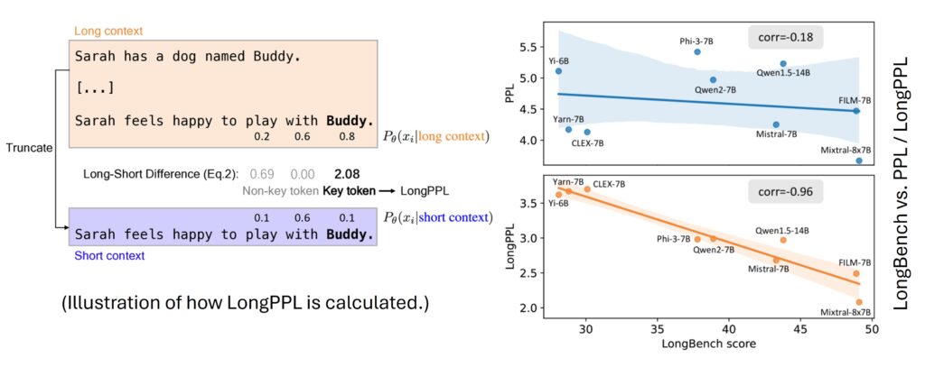
2. Context-Dependent Tokens: Compare the likelihood of a token given the full text vs. a truncated text.
   • If $P(w_i \mid \text{Full Context}) \gg P(w_i \mid \text{Short Context})$, then $w_i$ is a key token.
   • This differential (often called Long-Short Difference) isolates the specific benefit of the long window.

Takeaway: If you are evaluating a RAG system or long-context model, do not rely on standard sliding-window perplexity. Use a focused metric that targets the specific retrieval-dependent tokens.

Conclusion

To wrap up, Perplexity is the “Branching Factor” of your model. It tells you how confused the model is when predicting the next token.

• Use it for: Tracking training progress and comparing models on identical datasets/tokenizers.
• Do not use it for: Assessing generation quality (chat, reasoning) or long-context retrieval performance.

When in doubt, remember: A lower perplexity means the model is less surprised by the text, but it does not guarantee the model is smart.