
Imagine trying to understand a person’s life story just by looking at their credit card statements. You would see transactions—purchases, dates, and amounts—but you would miss the context, the relationships, and the “why” behind the data. You would have a list of facts, but not a narrative. A traditional database often gives you this fragmented view.
A knowledge graph (KG), on the other hand, is like building a rich, interconnected biography. It does not just store isolated facts; it weaves them together into a story. It connects entities (like people, products, or companies) through meaningful relationships (like works_at, is_friends_with, or has_purchased), creating a network of knowledge that is far more powerful than the sum of its parts.
Knowledge graphs are like rich, structured maps of how things in the world relate to each other.

Think of a KG as a digital brain for your data. Instead of looking up rows in tables, you are walking paths in a network of meaning. This lets you ask complex questions, discover hidden patterns, and reason about the world in a way that is both intuitive and powerful.
This write-up will guide you through the world of knowledge graphs, from core intuitions to practical applications. We will explore:
- The Big Idea: What a knowledge graph is and why it is more than just another database.
- The Building Blocks: How KGs are represented (RDF vs. Property Graphs).
- The Language of Graphs: Core concepts like entities, relations, and ontologies.
- From Raw Data to Rich Knowledge: A step-by-step guide to building your own KG.
- Making Graphs Smart: How machine learning (like KG embeddings and GNNs) brings predictive power to graphs.
- Real-World Impact: Practical applications and design principles.
The goal is to start with intuition, then layer in the formalism and implementation details, so that by the end you can both explain KGs to a non-technical colleague and design one for a real system.
What Is a Knowledge Graph?
The Intuitive View: From Data Points to a Network of Knowledge
A knowledge graph (KG) transforms data from a list of facts into a flexible, queryable network. It represents knowledge with three main components:
- Nodes (or Vertices): These are the “nouns” of your world—the entities. An entity can be a person (
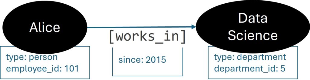
Alice), a place (San Francisco), a concept (Data Science), or an event (Product Launch 2024). - Edges (or Relationships): These are the “verbs” that connect your nouns. They describe how entities relate to one another, such as
Alice—[works_at]→Acme Corp, orDrug A—[treats]→Disease B. - Attributes (or Properties): This is extra information attached to nodes and edges. For example, the
Alicenode could have an attributerole: "Data Scientist", and theworks_atedge could have an attributesince: 2020.
Let us visualize this. Imagine you have two simple tables in a database:
| employee_id | name | department_id |
|---|---|---|
| 101 | Alice | 5 |
| dep_id | name |
|---|---|
| 5 | Data Science |
A knowledge graph merges this into a single, intuitive picture:
This simple shift in perspective unlocks powerful capabilities:
- Schema Flexibility: Want to add a new relationship, like
Alice—[mentors]→Bob? You just add a new edge. There is no need to redesign a rigid table schema. - Rich, Deep Queries: You can ask questions that would be complex and slow in a traditional database, like “Find all employees who work in the same department as Alice’s collaborators from last year.”
- Natural Explanations: The paths in a graph provide clear, human-readable explanations for a result. For example, a recommendation engine can explain why it suggested a product by showing the path: “You bought Product A, which is often bought with Product B.”
The Formal View: A World of Triples
Formally, a knowledge graph is often described as a directed labeled graph. The most fundamental representation is the triple, which consists of a (head, relation, tail), often abbreviated as \((h, r, t)\).
For example, the statement “Alice works at Acme” becomes the triple: (Alice, works_at, Acme).
A knowledge graph \(G\) can be defined as a collection of these triples:
$$ G = {(h, r, t) \mid h, t \in V, r \in R} $$
where:
- \(V\) is a set of entities (nodes).
- \(R\) is a set of relation types (edge labels), such as
works_at,cites,part_of.
How Knowledge Graphs Are Represented: RDF vs. Property Graphs
In the wild, knowledge graphs are primarily built using one of two models: the Resource Description Framework (RDF) model or the Property Graph model. The choice between them depends on your goals, whether you prioritize standardization and formal logic or developer-friendliness and performance.
RDF (Resource Description Framework): The Standard for Linked Data
The RDF model is the foundation of the Semantic Web, a W3C standard designed for data interoperability. Its core principle is that everything is represented as a triple:
$$ (\text{subject}, \text{predicate}, \text{object}) $$
This is the same (head, relation, tail) structure we saw earlier. For example:
(ex:Alice, ex:worksAt, ex:Acme)(ex:Acme, ex:locatedIn, ex:SanFrancisco)
Key characteristics of RDF:
- Uniformity: Everything is a triple. If you want to add an attribute, like the year Alice started working, you must model it with another triple. This can feel cumbersome but is highly consistent.
- Global Identifiers (URIs): Every entity and predicate is identified by a Unique Resource Identifier (URI), like a web URL. For example,
ex:Alicemight behttp://example.org/people/Alice. This prevents ambiguity and makes it easy to link datasets together. - Standards-Driven: RDF is supported by a mature stack of technologies, including SPARQL (a query language for graphs) and OWL/RDFS (languages for defining schemas and ontologies).
Choose RDF when:
- You are building for the open web or integrating data across different organizations (Linked Open Data).
- Formal logical reasoning and semantic consistency are critical.
- You need to adhere to established web standards.
Property Graphs: The Developer-Friendly Model
Property graphs are the model used by most popular graph databases today (like Neo4j and TigerGraph). They offer a more intuitive and flexible way to model data by allowing you to add properties (key-value pairs) directly to nodes and edges.
Using our example:
- Node: A node representing Alice could be stored as a single object with multiple properties:
{id: 1, label: "Person", name: "Alice", employee_id: 101, role: "Data Scientist"}. - Edge: The relationship between Alice and Acme could be an edge object with its own properties:
{from: 1, to: 2, label: "works_at", since: 2020}.
Key characteristics of Property Graphs:
- Intuitive and Flexible: Storing attributes directly on nodes and edges feels natural to developers and often leads to simpler, faster queries for attribute-heavy tasks.
- Performance-Oriented: The model is optimized for “graph traversal” queries—hopping from node to node across the network.
- Rich Ecosystem: Supported by popular graph databases and query languages like Cypher (declarative), GQL and Gremlin (programmatic).
Choose Property Graphs when:
- You are building a specific application and need high performance for complex graph queries.
- Your data model has many attributes on both nodes and edges.
- Developer productivity and ease of use are top priorities.
Choosing a Representation
Rough guidance:
- RDF: more suitable when you need semantic web standards, ontology reasoning, and data sharing.
- Property graphs: more suitable for application development, graph traversal queries, and operational workloads.
A useful mental model is: RDF is the logic and interoperability layer, property graphs are the product and engineering layer. Many real systems blend both: store the KG in a property graph for operations and expose parts in RDF for integration and semantics.
Core Concepts: Entities, Relations, Ontologies, and Reasoning
Entities and Relations
At the heart of a knowledge graph:
- Entity: a thing in the domain of interest.
- Examples:
User,Product,Paper,Disease,City.
- Examples:
- Relation: a directed, semantically meaningful connection between two entities.
- Examples:
purchased,cites,located_in,treats,collaborated_with. - Relations can have different structural properties:
- Functional vs. many-to-many:
born_inis almost functional;collaborated_withis many-to-many. - Symmetric:
married_tois symmetric;parent_ofis not. - Transitive:
part_ofandsubclass_ofrelations are often transitive.
- Functional vs. many-to-many:
- Examples:
Understanding these properties is important for both logical reasoning and machine learning models.
Ontology and Schema: The Blueprint for Your Knowledge
An ontology (or schema) defines the vocabulary and rules for your knowledge graph, ensuring that data is consistent, meaningful, and machine-readable.
An ontology specifies:
- Classes (or Types): The categories of entities in your graph. Examples:
Person,Organization,Product,Disease. - Relationships (or Predicates): The types of edges that can exist and which classes they can connect. For example, a
works_atrelationship connects aPersonto anOrganization. - Constraints and Axioms: The rules that govern your data.
- Domain and Range: The
works_atrelation must have aPersonas its subject (domain) and anOrganizationas its object (range). - Subclass Hierarchies: A
Researcheris a subclass ofPerson(Researcher ⊆ Person). This means any fact about aPersoncan be inherited by aResearcher. - Cardinality: A
Personcan have exactly onebirth_date.
- Domain and Range: The
Why is an ontology so important? It enables:
- Data Consistency: It prevents nonsensical data from entering your graph, like a
Productbeing the CEO of aCompany. - Automated Reasoning (Inference): It allows the system to infer new facts from existing ones. If you know that
Researcher ⊆ PersonandAliceis aResearcher, the system can automatically infer thatAliceis also aPerson.
Reasoning: Deriving New Knowledge from Old Facts
Reasoning is the process of using the rules in your ontology to automatically derive new information that is not explicitly stated in the data. It is like a detective using a set of rules to solve a case.
Reasoning systems typically distinguish between:
- TBox (Terminological Box): The schema (classes, relations, axioms) or ontology—your set of rules and definitions (e.g.,
All Researchers are People). - ABox (Assertional Box): The instance data (entities and concrete facts)—your collection of observed facts (e.g.,
Alice is a Researcher).
Common reasoning tasks include:
- Type Inference: If
Alicehas authored many papers and works at a university, the system might infer thatAliceis aResearcher, even if it was never explicitly stated. - Relation Inference: If the graph knows that
co-authoris a symmetric relation, and it sees the fact(Alice, co-author, Bob), it can infer(Bob, co-author, Alice). - Constraint Checking: The system can flag violations of the ontology, such as a
Personhaving two different birth dates.
In practice, full-blown logical reasoning can be computationally expensive. Many production systems use a mixture of:
- Lightweight reasoning (RDFS, simple rules).
- Precomputed inferences.
- Machine learning to suggest likely but uncertain facts.
How to Build a Knowledge Graph: A Step-by-Step Narrative
Building a knowledge graph is not just a technical task; it is an act of knowledge modeling. You are deciding how the world should be described for a particular purpose.
Let us walk through the process with a story. Imagine we want to build a knowledge graph for movie recommendations, a “Movieverse KG.”
Step 1: Start with the “Why”—Define Your Use Cases
Before writing any code, we ask: “What questions should our Movieverse KG be able to answer?”
- Goal 1 (Simple Recommendation): “If a user likes Inception, what other movies should they watch?”
- Goal 2 (Content-Based Filtering): “Show me all science fiction movies directed by Christopher Nolan.”
- Goal 3 (Collaborative Filtering): “Recommend movies that people with similar tastes to mine have enjoyed.”
These questions will guide every decision we make, from the data we need to the structure of our ontology.
Step 2: Gather Your Ingredients—Identify Data Sources
Next, we hunt for data. Our sources are scattered and diverse:
- Internal Database: A SQL database with tables for
movies,users, andratings. - Unstructured Text: Movie synopses and reviews stored as text files.
- External APIs: Public APIs like IMDb or TMDb that provide rich metadata (cast, crew, genres, etc.).
Step 3: Find the Nouns—Entity Extraction and Linking
This is where we start reading the data and identifying the key entities.
- Named Entity Recognition (NER): We run an NER model on movie synopses. From the text “Leonardo DiCaprio stars as a thief…”, the model identifies “Leonardo DiCaprio” as a
Person. - Entity Linking (EL): Is “Christopher Nolan” the same person in our database, in a review, and in the IMDb API? Entity Linking is the crucial step of disambiguating and merging these mentions into a single, canonical node in our graph (e.g.,
entity:nm0634240). - Canonicalization: We unify different names like “Leo DiCaprio” and “Leonardo Wilhelm DiCaprio” to point to the same entity.
Step 4: Find the Verbs—Relation Extraction
Now we connect our entities. We look for relationships in the data:
- From Structured Data: A
ratingstable with(user_id, movie_id, rating)directly gives us(User)—[rated]→(Movie)edges with the rating as a property. - From Text: From the sentence “Christopher Nolan directed the movie Inception,” a relation extraction model extracts the triple:
(Christopher Nolan, directed, Inception).
Techniques for this can range from simple text patterns (e-g., looking for the word “directed by”) to sophisticated machine learning models trained to classify the relationship between two entities in a sentence.
Step 5: Create the Blueprint—Schema Alignment and Normalization
As we pull in data from different sources, it is often messy and inconsistent. This step is about cleaning it up.
- Schema Alignment: We map the fields from our sources to our ontology. The
movies.titlefrom our database, theoriginal_titlefrom the API, and thenamefrom a text mention all get mapped to theMovie.titleproperty in our KG. - Value Normalization: We standardize values. Movie runtimes are all converted to minutes, release dates are set to
YYYY-MM-DDformat, and genre names are standardized (e.g., “Sci-Fi” and “Science-Fiction” both becomeScienceFiction). - Entity Resolution: We merge duplicate nodes. If we accidentally created two separate nodes for “Christopher Nolan,” this is where we would merge them into one, combining all their relationships.
Step 6: Build the Library—Storage and Indexing
Finally, we choose a home for our KG. Based on our needs, we might select:
- A Graph Database (like Neo4j, JanusGraph, TigerGraph): Optimized for the kind of “who-likes-what” traversal queries we need for recommendations.
- A Triple Store (like Blazegraph, GraphDB, Amazon Neptune): A good choice if we plan to share our movie data with other organizations and need strong standards compliance.
- Graph layers on top of big data systems (Apache Spark GraphFrames, graph libraries on top of column stores): Useful when the KG is part of a larger analytics or batch processing stack.
Once stored, the data is indexed to ensure that queries like “Find all movies starring Tom Hanks” are fast and efficient. The result is a living, breathing Movieverse KG, ready to power our recommendation engine.
At this point, it is helpful to sanity-check your design against how the graph will actually be used:
- Query patterns: Do you need deep traversals, aggregates, subgraph matching, or path queries?
- Latency vs throughput: Do you need low-latency online serving, or is this primarily for offline analytics?
- Updates: How frequently does the graph change? Do you support streaming updates or batch rebuilds?
Querying a Knowledge Graph
Once you have a KG, you want to ask it complex questions.
Pattern-Based Queries
In a graph database, a typical query finds patterns in the graph: “a user who purchased a product that another user also purchased.”
Example (in Cypher-like pseudocode):
MATCH (u:User)-[:PURCHASED]->(p:Product)<-[:PURCHASED]-(v:User)
WHERE u.id = "user_123" AND u <> v
RETURN DISTINCT v AS similar_customers
This finds users who purchased the same products as a given user.
Semantic Queries (SPARQL)
In RDF, SPARQL is the standard query language. It matches triples based on patterns and filters.
Conceptually, you describe a small graph pattern and ask the system to find all matches in the larger graph.
Example pattern: “Find drugs that treat a disease and have a certain side effect.” This becomes a graph pattern over triples (drug, treats, disease) and (drug, has_side_effect, effect).
Path Queries and Explanations
One of the strengths of KGs is the ability to explain answers via paths:
- For recommendation: “We recommend Product X because it is frequently co-purchased with Product Y, which you bought, and both are alternatives to Product Z.”
- Technically, this is a path like
You→purchased→Y→co_purchased_with→X.
These paths can be surfaced in user interfaces to improve transparency and trust.
Machine Learning with Knowledge Graphs
Knowledge graphs and machine learning reinforce each other. The KG provides rich structure; ML can fill in gaps, denoise data, and generate predictions.
Knowledge Graph Embeddings
Knowledge graph embeddings map entities and relations into continuous vector spaces. The core idea is to represent each entity and relation as a vector. These vectors are then fine-tuned so that the relationships observed in the KG are preserved as mathematical relationships in the vector space.
- Each entity \(e \in V\) has an embedding \(\mathbf{e} \in \mathbb{R}^d\).
- Each relation \(r \in R\) has a parameterization (a vector, matrix, or more complex operator).
The model assigns a score \(f(h, r, t)\) to each triple \((h, r, t)\), where higher scores mean more plausible facts.
Common families of models:
- Translational models (e.g., TransE):
- Model relations as translations in embedding space.
- Intuition: for a valid triple \((h, r, t)\), we want: $$ \mathbf{h} + \mathbf{r} \approx \mathbf{t} $$
- The score function often uses a distance metric: $$ f(h, r, t) = -|\mathbf{h} + \mathbf{r} – \mathbf{t}| $$
- If you start at the vector for
Parisand add the vector foris_capital_of, you should land very close to the vector forFrance. - The TransE model is trained by rewarding it for making this equation true for valid triples and penalizing it when it is true for invalid ones (a process called negative sampling).
- Bilinear Models (e.g., DistMult, ComplEx): These models use multiplicative interactions, like dot products, to score triples. They are better at handling more complex relation patterns, such as symmetry (e.g.,
is_married_to). For example, DistMult scores a triple like this: $$ f(h, r, t) = \mathbf{h}^\top \text{diag}(\mathbf{r}) \mathbf{t} $$
Use Cases for KG Embeddings
- Link prediction: predict missing edges (e.g., which drug likely treats which disease, or which user is likely to purchase which product).
- Entity similarity: find similar entities by vector distance.
- Feature inputs: feed KG embeddings into downstream models (e.g., recommenders, classifiers).
- Clustering and visualization: group similar entities or visualize the graph structure in lower dimensions.
Graph Neural Networks (GNNs) on Knowledge Graphs
While KG embeddings learn a single, static vector for each entity, Graph Neural Networks (GNNs) create dynamic, context-aware embeddings. A GNN learns about a node by looking at its local neighborhood in the graph.
The core intuition behind GNNs is message passing. Each node in the graph sends “messages” to its neighbors, and each node updates its own representation by “listening” to the messages it receives.
- Each node starts with an initial embedding (features, text encodings, or learned vectors).
- GNN layers aggregate information from neighbors to update each node representation. This process is repeated for several layers, allowing each node’s embedding to capture information from further and further out in the graph.
Formally, a GNN layer can be described as an aggregation and update step:
$$
\mathbf{h}_v^{(k)} = \sigma\left( W^{(k)} \cdot \text{AGGREGATE}\{ \mathbf{h}_u^{(k-1)} : u \in \mathcal{N}(v) \} \right)
$$
where:
- \(\mathbf{h}_v^{(k)}\) is the embedding of node \(v\) at layer \(k\).
- \(\mathcal{N}(v)\) is the set of neighbors of node \(v\).
- \(\text{AGGREGATE}\) is a function that combines the messages from the neighbors (e.g., by summing or averaging them).
- \(W^{(k)}\) is a learnable weight matrix that transforms the aggregated message.
- \(\sigma\) is a nonlinearity (like ReLU).
Example:
Imagine node \(v\) is Alice. Her neighbors are Acme (where she works) and Bob (who she mentors).
- Message Passing:
Acmesends a message (its current vector representation) toAlice.Bobdoes the same. - Aggregation:
Alice‘s node takes these two vectors and averages them. This average vector represents the “context” of her surroundings. - Update: This context vector is multiplied by a weight matrix \(W\) (which the model learns during training) and passed through an activation function. The result is
Alice‘s new embedding, which now contains information about her workplace and mentee.
For knowledge graphs with different types of relationships, specialized GNNs like the Relational Graph Convolutional Network (R-GCN) use different weight matrices for each relation type. This allows the model to learn, for example, that the message from a works_at edge should be treated differently from the message from a purchased edge.
GNNs are powerful for:
- Node Classification: Predicting a label for a node, like the category of a product or the risk profile of a customer.
- Link Prediction: Predicting missing edges with high accuracy, as the model has access to rich neighborhood information.
- Graph-Level Tasks: Classifying an entire graph, such as determining if a molecule is toxic.
Integrating Text and KGs
Many modern systems combine textual representations (from language models) with KGs:
- Use a language model (e.g., a transformer) to embed descriptions of entities.
- Combine text embeddings with KG structure via GNNs or joint training.
- Use KGs as a retrieval and grounding layer for LLMs (retrieval-augmented generation, tool-augmented reasoning).
This hybrid approach is particularly useful when you have both rich unstructured text and structured knowledge.
Practical Example: A Mini KG in Python with networkx
While production knowledge graphs run on specialized databases, you can build a simple one in Python using the networkx library. This is a great way to solidify the core concepts before worrying about clusters and query optimizers.
Let us create a tiny KG representing a few entities and relationships.
import networkx as nx
import matplotlib.pyplot as plt

# Create a directed graph, the foundation of our KG
G = nx.DiGraph()

# --- Step 1: Add entities (nodes) with attributes ---
# The nodes are the "nouns" of our world.
# Attributes are key-value pairs that describe the node.
G.add_node("Alice", type="Person", role="Data Scientist")
G.add_node("Acme", type="Organization", industry="Retail")
G.add_node("ProductX", type="Product", category="Electronics")
G.add_node("Bob", type="Person", role="Software Engineer")

# --- Step 2: Add relationships (edges) with attributes ---
# The edges are the "verbs" connecting our nouns.
# We can add attributes to edges to provide more context.
G.add_edge("Alice", "Acme", relation="works_at", since=2020)
G.add_edge("Bob", "Acme", relation="works_at", since=2022)
G.add_edge("Alice", "ProductX", relation="purchased", timestamp="2024-05-01")
G.add_edge("Alice", "Bob", relation="collaborates_with")

# --- Step 3: Query the graph ---
# Queries involve traversing the graph to find patterns.

# Query 1: Who works at Acme?
employees = [
    u for u, v, data in G.edges(data=True)
    if v == "Acme" and data.get("relation") == "works_at"
]
print(f"Employees at Acme: {employees}")  # Output: ['Alice', 'Bob']

# Query 2: What products has Alice purchased?
products_purchased = [
    v for u, v, data in G.edges(data=True)
    if u == "Alice" and data.get("relation") == "purchased"
]
print(f"Products purchased by Alice: {products_purchased}")  # Output: ['ProductX']

# This toy example demonstrates the core ideas:
# 1. Nodes are entities with properties.
# 2. Edges are relationships, also with properties.
# 3. Queries are graph traversals that match patterns.

# Optional: Visualize the graph to see the structure
pos = nx.spring_layout(G, seed=42)
nx.draw(G, pos, with_labels=True, node_size=2000, node_color='lightblue', font_size=10)
edge_labels = nx.get_edge_attributes(G, 'relation')
nx.draw_networkx_edge_labels(G, pos, edge_labels=edge_labels)
plt.title("A Simple Knowledge Graph")
plt.show()This simple script captures the essence of a property graph. In a real-world system, you would use a dedicated graph database that can handle billions of nodes and edges and provide a powerful query language like Cypher or SPARQL, but the underlying concepts are the same.
Applications of Knowledge Graphs
Knowledge graphs are used across many domains. A non-exhaustive list:
- Search and question answering:
- Powering knowledge panels in web search.
- Supporting semantic search: query expansion, intent understanding, and result ranking.
- Recommendation systems:
- User–item–content graphs for recommendations that leverage multi-hop relationships.
- Explainable recommendations via paths (e.g., “because you liked this author and this topic”).
- Enterprise data integration:
- Unifying silos: CRM, ERP, HR, analytics systems into a single, connected view.
- Supporting master data management and 360-degree views (customer, product, asset).
- Biomedical and scientific discovery:
- Drug–target–disease graphs for drug repurposing.
- Citation and collaboration graphs for literature discovery.
- Fraud detection and risk analysis:
- Transaction and entity graphs for detecting anomalous patterns.
- Network-based risk scoring (e.g., businesses connected to high-risk entities).
Design Considerations and Best Practices
Start from Questions, Not from Data
It is tempting to ingest all available data and “see what happens”. A better approach:
- Start from a small set of concrete, high-value questions.
- Derive the initial ontology from these questions.
- Iteratively expand the KG and ontology as new questions arise.
Balance Expressivity and Simplicity
Highly expressive ontologies (many classes, relations, and constraints) increase modeling power but also complexity.
Practical strategies:
- Keep the core ontology small and stable.
- Use extension namespaces or modules for experimental or domain-specific concepts.
- Avoid over-modeling rare edge cases early on.
Data Quality and Provenance
Knowledge graphs often integrate noisy sources. Track:
- Confidence scores on edges and nodes.
- Provenance: where did a fact come from (system, model, human)?
- Timestamps: when was a fact observed or valid?
This enables downstream systems to filter, debug, and reason under uncertainty.
Human-in-the-Loop Curation
Even with strong ML, human experts are invaluable for:
- Reviewing and correcting important parts of the KG.
- Defining and refining ontologies.
- Adding high-value facts and rules that models might miss.
Tools for browsing, editing, and annotating the KG are essential.
Integration with Machine Learning Pipelines
For ML practitioners, it is useful to treat the KG as:
- A feature source: generate graph-based features (node centrality, community membership, multi-hop counts).
- A label source: derive supervision signals (e.g., target relations, categories).
- A constraint source: enforce consistency (e.g., impossible relations) in models.
Designing APIs and data flows that make the KG accessible from ML training and serving pipelines significantly increases its value.
Summary and Next Steps
- A knowledge graph is a powerful way to represent data as a network of entities and relationships, moving beyond simple tables to capture rich context.
- It is like a “digital brain” for your data, enabling deep queries and intuitive explanations.
- The two main models are RDF (standardized, for open data) and Property Graphs (developer-friendly, for applications).
- Building a KG is a systematic process: define use cases, integrate data, extract entities and relations, and load into a specialized database.
- Machine learning supercharges KGs. KG embeddings learn vector representations for link prediction, while GNNs create context-aware embeddings by learning from a node’s neighborhood.
- KGs are the backbone of many intelligent systems, including search engines, recommendation systems, and fraud detection platforms.
Where to go from here?
- Get Your Hands Dirty: Use a library like
networkxto model a domain you are interested in—your favorite books, a project at work, or a historical event. - Explore a Graph Database: Download a free version of a graph database like Neo4j and complete their tutorials. You will quickly see the power of a real graph query language.
- Dive into the ML: Implement a simple KG embedding model like TransE on a benchmark dataset (e.g., WordNet). This will give you a deep appreciation for how these models learn.
The key takeaway is this: knowledge graphs provide the structure, and machine learning provides the intelligence. Together, they form a powerful combination for building the next generation of data-driven applications.

Happy is a seasoned ML professional with over 15 years of experience. His expertise spans various domains, including Computer Vision, Natural Language Processing (NLP), and Time Series analysis. He holds a PhD in Machine Learning from IIT Kharagpur and has furthered his research with postdoctoral experience at INRIA-Sophia Antipolis, France. Happy has a proven track record of delivering impactful ML solutions to clients.
Subscribe to our newsletter!