How to Choose the Best Learning Rate Decay Schedule for Your Model

The training process involves optimizing a model’s parameters to minimize the loss function. One crucial aspect of this optimization is the learning rate (LR) which dictates the size of the steps taken towards the minimum of the loss function. A well-chosen learning rate can lead to faster convergence and better performance, whereas a poorly chosen one can cause the training process to either converge too slowly or diverge entirely.

Learning rate decay is an essential technique that involves systematically decreasing the learning rate throughout the training process.

This article provides a comprehensive understanding of learning rate decay, its importance, and the various methods used to implement it.

What is Learning Rate?

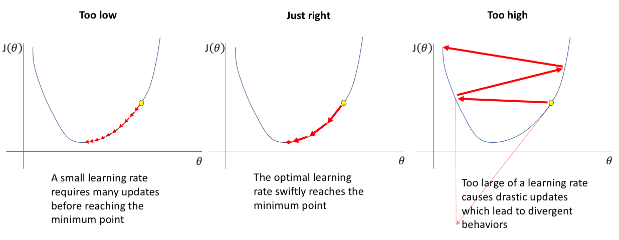
The learning rate is a hyperparameter that controls how much to change the model in response to the estimated error each time the model weights are updated. Choosing an appropriate learning rate is critical:

• Too High: If the learning rate is too large, the model may converge too quickly to a suboptimal solution or diverge entirely. This can lead to oscillating behavior or a complete failure to converge.
• Too Low: Conversely, if the learning rate is too small, the training process can become excessively slow, requiring many more iterations to reach a satisfactory solution.

What is Learning Rate Decay?

Learning rate decay refers to the gradual reduction of the learning rate as training progresses. The rationale behind this approach is based on the intuition that:

1. Exploration Early on: At the beginning of training, a higher learning rate can help traverse the loss surface more effectively, allowing the model to escape local minima and explore a broader area.
2. Precision Late in Training: As the model starts to converge, it can benefit from smaller adjustment sizes to fine-tune the weights, avoiding overshooting the minimum.

In its simplest form, learning rate decay helps balance between exploration during the initial stages of training and exploitation during later stages, optimizing convergence speed and accuracy.

Why Use Learning Rate Decay?

1. Avoid Overshooting: With a higher learning rate, there’s a risk of overshooting the minimal point of the loss function, especially in complex landscapes. Learning rate decay helps to mitigate this by reducing the step sizes later in training.
2. Improved Convergence: Decaying the learning rate can ensure that the optimization process converges to a better local minimum as it allows the algorithm to take smaller steps when it is close to the optimal parameters.
3. Smoother Training Process: Gradually reducing the learning rate can lead to a more stable and smoother training process, helping mitigate fluctuations in the loss.
4. Regularization: Sometimes, higher learning rates can lead to overfitting. Reducing the learning rate can help regularize training, promoting a more generalizable model.

Common Methods of Learning Rate Decay

1. Time-Based Decay (Linear Decay)

This method, also known as linear decay, linearly decreases the learning rate over time. The equation is:

lr(t) = lr(0) / (1 + decay_rate * t)

Where:

• lr(t): Learning rate at time step t (often epochs or iterations).
• lr(0): Initial learning rate.
• decay_rate: A hyperparameter controlling the decay rate.
• t: Time step (epoch or iteration).

Time-based decay is straightforward to implement but can be overly aggressive initially and too slow later, potentially hindering performance for complex models.

2. Step Decay

Step decay involves reducing the learning rate by a constant factor at predefined intervals (steps). The equation can be represented as:

lr(t) = lr(0) * drop_rate ^ floor(t / drop_every)

Where:

• lr(t): Learning rate at time step t.
• lr(0): Initial learning rate.
• drop_rate: The factor by which the learning rate is multiplied at each drop (e.g., 0.5 for halving).
• drop_every: The number of time steps (epochs or iterations) between each drop.
• floor(): The floor function, which rounds down to the nearest integer.

Step decay is simple to implement but requires careful tuning of drop_rate and drop_every.

3. Exponential Decay

Exponential decay reduces the learning rate exponentially over time. The equation is:

lr(t) = lr(0) * decay_rate ^ t

Where:

• lr(t): Learning rate at time step t.
• lr(0): Initial learning rate.
• decay_rate: A hyperparameter between 0 and 1 controlling the decay rate.

Exponential decay offers a smoother reduction than time-based decay, often proving more suitable for complex models.

4. Polynomial Decay

Polynomial decay reduces the learning rate according to a polynomial function. The equation is:

lr(t) = lr(0) * (1 - t / T)^power

Where:

• lr(t): Learning rate at time step t.
• lr(0): Initial learning rate.
• t: Current time step (epoch or iteration).
• T: Total number of time steps (total epochs or iterations).
• power: A hyperparameter controlling the shape of the decay curve.

Polynomial decay provides greater flexibility in shaping the decay compared to other methods.

5. Cosine Annealing

Cosine annealing follows a cosine function to vary the learning rate. It starts with a high learning rate, decreases it to a minimum, and then increases it again, repeating this cycle. The equation for a single cycle is:

lr(t) = lr_min + 0.5 * (lr_max - lr_min) * (1 + cos(pi * t / T))

Where:

• lr(t): Learning rate at time step t.
• lr_min: Minimum learning rate.
• lr_max: Maximum learning rate (often the initial learning rate).
• t: Current time step within the cycle.
• T: Total number of time steps in the cycle.

Cosine annealing encourages exploration of different parts of the solution space and can lead to improved optima.

Cyclical Learning Rates (CLR)

While not strictly a decay method, Cyclical Learning Rates (CLR) deserve mention. They involve cyclically varying the learning rate between lower and upper bounds. This can be implemented with various functions, including triangular and sinusoidal cycles. The idea is to periodically increase the learning rate to escape sharp minima and explore broader regions of the loss landscape.

Choosing the Right Learning Rate Decay Method

The choice of learning rate decay strategy often depends on the specific model architecture, the dataset, and even the computational resources available. It is essential to experiment and track performance using different decay strategies. Here are some guidelines:

• Start simple: Begin with step or exponential decay.
• Monitor training: Observe the training process and adjust decay parameters accordingly.
• Complex models: Consider cosine annealing or CLR for more complex scenarios.
• Visualize: Plot the learning rate curve to understand its behavior.

References

• Jeremy Jordan’s blog
• datacamp tutorial
• medium article