In the world of machine learning, especially when dealing with structured or tabular data, few algorithms have achieved the level of dominance and respect as Gradient Boosting. It has been the secret sauce behind countless victories in data science competitions, like those on Kaggle, and a reliable workhorse in many industrial applications.
But what makes it so powerful? Imagine you are assembling a team of specialists to solve a complex problem. Instead of having them all work in parallel and hoping their combined knowledge is enough, you decide on a different strategy. You have the first specialist create an initial solution. Then, you have a second specialist look at the mistakes the first one made and focus exclusively on correcting those errors. A third specialist then corrects the remaining mistakes of the combined team, and so on. Each new member does not just add knowledge; they specifically target the weaknesses of the group. This is the core intuition behind Gradient Boosting.
It is an ensemble technique that builds a single, strong predictive model by sequentially adding weaker models, where each new model is trained to correct the errors made by the previous ones.
The Intuition: Learning from Mistakes
At its heart, GradientBoosting is a step-by-step process. Let us walk through a simple regression example to build our intuition.
- Start with a Simple Model: We begin by making an initial, simple prediction for all our data points. This could be the average value of the target variable. This first model is often called a “weak learner” because it is not very accurate on its own.
- Calculate the “Mistakes”: We then calculate the errors made by this initial model. In a simple regression case, these errors are the residuals—the difference between the actual values and our model’s predictions.
- Train a New Model on the Mistakes: Here is the clever part. We train a new weak learner (typically a small decision tree) not on our original target variable, but on the residuals from the previous step. The goal of this new model is to learn the patterns in the mistakes.
- Combine the Models: We update our predictions by adding the predictions from this new model (scaled by a small number called the learning rate) to our previous predictions. This new set of combined predictions should be more accurate than before.
- Repeat: We repeat steps 2-4: calculate the new residuals, train another model on these new residuals, and add it to our ensemble. We continue this process for a specified number of iterations, with each new model incrementally improving the overall performance by focusing on the data points that are still hard to predict.
The “Gradient” in Gradient Boosting: The Mathematical Core
The intuitive idea of “correcting mistakes” is powerful, but to make it a flexible algorithm that can handle any task (regression, classification, etc.), we need a more formal framework. This is where the “gradient” comes in.
Instead of thinking in terms of simple residuals, we think in terms of a loss function which is a measure of how bad our model’s predictions are. For regression, a common loss function is Mean Squared Error (MSE). For classification, it might be Log-Loss. The goal is always to find a model that minimizes this loss function.
Gradient Boosting is an application of gradient descent in the space of functions. Instead of updating numerical parameters to minimize a loss, we are updating a model to minimize a loss.
Here is the general algorithm:
- Initialize the model with a constant value: $$F_0(x) = \arg\min_{\gamma} \sum_{i=1}^{n} L(y_i, \gamma)$$ This is our initial simple prediction, like the mean for MSE loss. For every data point from \(i=1,…,n\), calculate the loss between the true value \(y_i\) and our guess \(\gamma\), and then add all those losses together.
- For each iteration m (from 1 to M):
- Compute the pseudo-residuals: These are the negative gradients (the “direction of steepest descent”) of the loss function with respect to the previous model’s predictions, \(F_{m-1}(x)\).
$$r_{im} = – \left[ \frac{\partial L(y_i, F(x_i))}{\partial F(x_i)} \right]_{F(x)=F_{m-1}(x)}$$
For an MSE loss function, \(L(y, F) = \frac{1}{2}(y – F)^2\), the negative gradient is simply \((y – F)\), which is the standard residual. This is why our earlier intuition works perfectly for MSE! For other loss functions, it gives us a generalized notion of “error.” - Fit a weak learner (e.g., a decision tree) \(h_m(x)\) to the pseudo-residuals. This tree is trained to predict the direction that will best reduce our loss.
- Find the optimal step size \(\gamma_m\) for this new learner. We want to find the multiplier that minimizes our loss when we add the new tree to our ensemble.
$$\gamma_m = \arg\min_{\gamma} \sum_{i=1}^{n} L(y_i, F_{m-1}(x_i) + \gamma h_m(x_i))$$ - Update the model:
$$F_m(x) = F_{m-1}(x) + \nu \gamma_m h_m(x)$$
Here, \(\nu\) is the learning rate, a small constant (e.g., 0.1) that we introduce to prevent overfitting. This is also known as shrinkage.
- Compute the pseudo-residuals: These are the negative gradients (the “direction of steepest descent”) of the loss function with respect to the previous model’s predictions, \(F_{m-1}(x)\).
This process is repeated M times, resulting in a final model \(F_M(x)\) that is a powerful, additive combination of many weak learners.
$$F_M(x) = F_0(x) + \sum_{m=1}^{M} \nu \gamma_m h_m(x)$$
Scikit-Learn Example
Scikit-learn provides a straightforward implementation. Here is how you would use it for a regression problem:
import numpy as np
from sklearn.ensemble import GradientBoostingRegressor
from sklearn.model_selection import train_test_split
from sklearn.metrics import mean_squared_error

# 1. Generate some sample data
X = np.random.rand(100, 1) * 10
y = np.sin(X).ravel() + np.random.randn(100) * 0.1

# 2. Split data
X_train, X_test, y_train, y_test = train_test_split(X, y, test_size=0.2, random_state=42)

# 3. Initialize and train the model
# Key hyperparameters:
# n_estimators: The number of boosting stages (trees) to perform.
# learning_rate: Shrinks the contribution of each tree.
# max_depth: The maximum depth of the individual regression estimators.
gbr = GradientBoostingRegressor(n_estimators=100, learning_rate=0.1, max_depth=3, random_state=42)

gbr.fit(X_train, y_train)

# 4. Make predictions and evaluate
y_pred = gbr.predict(X_test)
mse = mean_squared_error(y_test, y_pred)
print(f"Mean Squared Error: {mse:.4f}")Practical Tips and Best Practices
Gradient Boosting is powerful, but it comes with several hyperparameters that need to be tuned to prevent overfitting and achieve the best performance.
n_estimatorsvs.learning_rate: These two are deeply connected. A lowerlearning_raterequires a highern_estimatorsto achieve the same level of training error. The trade-off is that a lower learning rate with more estimators is almost always more robust against overfitting. A common strategy is to set the learning rate to a small value (e.g., 0.01-0.1) and then use early stopping to find the optimal number of trees.- Tree-Specific Parameters (
max_depth,min_samples_split, etc.): These control the complexity of the individual weak learners. For Gradient Boosting, it is common to use very shallow trees, often with amax_depthbetween 3 and 8. This is because we want “weak” learners that each contribute a small amount to the final prediction, preventing any single tree from dominating. - Subsampling: Modern Gradient Boosting implementations (like in Scikit-learn, XGBoost, and LightGBM) use Stochastic Gradient Boosting. This means that each tree is trained on a random subsample of the data. This introduces randomness, reduces variance, and can significantly prevent overfitting. The
subsampleparameter controls the fraction of data to be used for fitting each tree. A value around 0.8 is often a good starting point. - Early Stopping: Instead of manually setting
n_estimators, it is better to train for a large number of trees and stop when the performance on a validation set no longer improves. This is a highly effective way to find the right number of iterations without overfitting to the training data. - Feature Importance: Gradient Boosting models provide a measure of feature importance, which tells you which features were most useful in making predictions. This can be a valuable tool for understanding your data and for feature selection.
Concluding Thoughts
Gradient Boosting is more than just another algorithm; it is a fundamental concept that combines several key ideas in machine learning: the wisdom of ensembles, the precision of gradient descent, and the power of iterative improvement. By building a model that learns from its mistakes in a structured, mathematically-grounded way, it has rightfully earned its place as one of the most effective and versatile tools in a data scientist‘s toolkit.

Happy is a seasoned ML professional with over 15 years of experience. His expertise spans various domains, including Computer Vision, Natural Language Processing (NLP), and Time Series analysis. He holds a PhD in Machine Learning from IIT Kharagpur and has furthered his research with postdoctoral experience at INRIA-Sophia Antipolis, France. Happy has a proven track record of delivering impactful ML solutions to clients.
Subscribe to our newsletter!