In the world of artificial intelligence, we have models that are experts at understanding text and others that are masters of interpreting images. But what if we could build a bridge between these two worlds? What if a model could understand images through the lens of human language? This is the revolutionary concept behind OpenAI’s CLIP (Contrastive Language-Image Pre-training) model.
Imagine showing a young child a picture book. You point to a picture of a furry, four-legged animal and say “dog.” You show them another picture of a different breed and say “dog” again. Over time, the child learns to associate the abstract concept and the word “dog” with the visual features of dogs. They can eventually identify a dog in a new picture, even if they have never seen that specific breed before.
CLIP learns in a conceptually similar way, but on a staggering scale. It is not just about recognizing a few objects; it is about creating a rich, shared space where visual and textual concepts coexist.
How Does CLIP Learn? An Intuitive Overview
At its core, CLIP is designed to solve a simple, intuitive task: given an image, which caption from a list of possible captions is the correct one? By training to solve this problem, it develops a profound understanding of both modalities.
The Power of Web-Scale Data
Instead of using meticulously curated and labeled datasets (like ImageNet, which requires specific labels like “tabby cat” or “golden retriever”), CLIP’s creators took a different approach. They scraped a massive dataset of 400 million (image, text) pairs from the internet. This text was not a clean label but whatever alt-text or caption was associated with the image. This noisy, diverse, and enormous dataset is a key ingredient to CLIP’s success, as it exposes the model to a vast range of objects, scenes, and concepts described in natural human language.
The Core Idea: A Matching Game
Think of the training process as a massive matching game. For any given batch of data, the model is presented with, say, 32 images and their 32 corresponding captions. The model’s job is to correctly predict which of the 32×32 possible pairings are the correct ones. To do this, it must learn to recognize that the image of a cat is semantically closer to the text “a photo of a cat” than it is to “a sunset over the ocean.”
Two Minds, One Goal: The Encoders
To play this matching game, CLIP uses a dual-encoder architecture. It has two separate models that work in tandem:
- Image Encoder: This model’s job is to look at an image and distill its visual essence into a single list of numbers, called an embedding. It learns to pick out key features—shapes, colors, textures, and the objects they form.
- Text Encoder: This model’s job is to take a piece of text and distill its semantic meaning into an embedding of the same size.
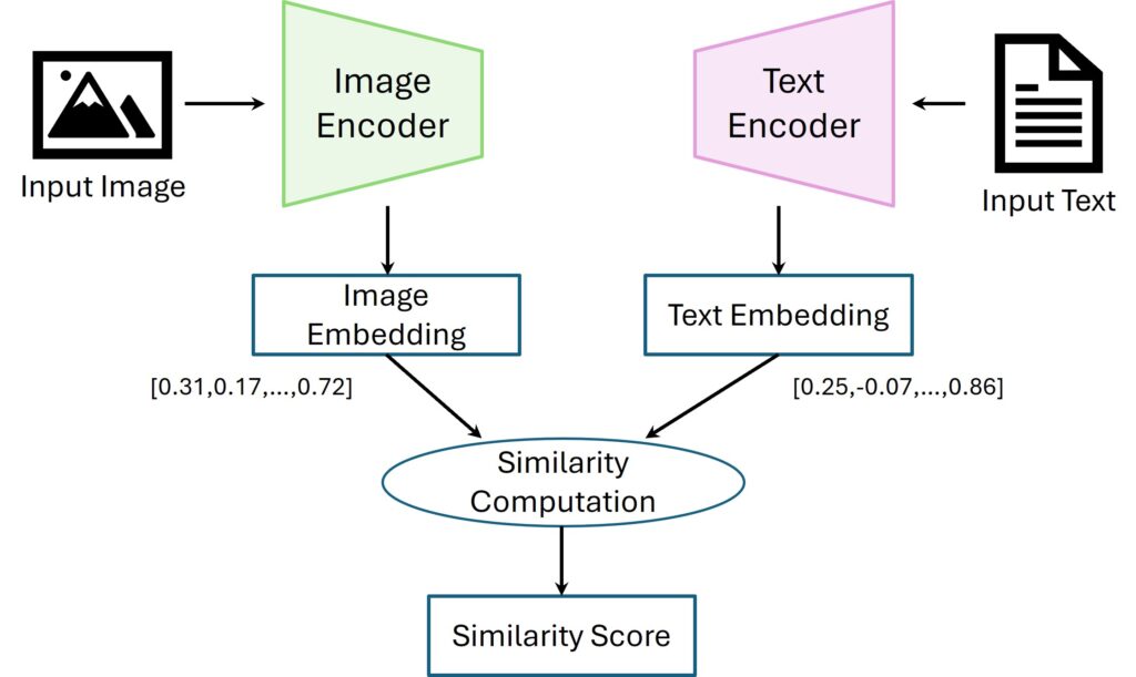
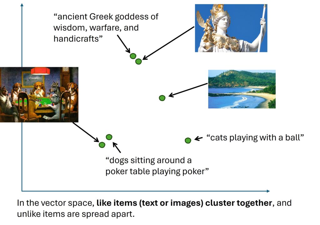
The magic of CLIP is that these two encoders are trained together. They learn to project their outputs into the same shared embedding space. In this space, the embedding for an image of a dog will be located very close to the embedding for the text “a picture of a dog.”
Key Breakthroughs:
- Task-Agnostic Learning: CLIP doesn’t require task-specific training data, making it adaptable to new challenges without fine-tuning. CLIP can classify images it has never seen before, using only natural language descriptions (Zero-Shot Image Classification).
- Scalability: Trained on 400 million (image, text) pairs, CLIP demonstrates how large-scale web data can drive AI advancements. CLIP maps both text and images to the same embedding space.
- Multimodal Understanding: By aligning images and text in a shared embedding space, CLIP excels at tasks ranging from OCR to action recognition.
A Deeper Dive: The Technical Architecture and Training
While the intuition is straightforward, the execution involves sophisticated deep learning components and a clever training objective.
The Architecture
- Image Encoder: CLIP’s authors experimented with several architectures, but the most effective ones were based on the Vision Transformer (ViT) (ViT-L/14) or ResNet variants (e.g., RN50x64). A ViT treats an image as a sequence of smaller patches, similar to how a language model treats a sentence as a sequence of words. This allows it to capture both local features and global context effectively. Modified with attention pooling and anti-aliased blur is used for better feature extraction.
- Text Encoder: For the text side, a standard Transformer model (63M parameters, with lower-cased BPE text) is used. It is a multi-layer model that uses self-attention mechanisms to build a rich representation of the input text’s meaning.
- Shared Embedding Space: The two encoders produce embeddings in a shared vector space (512 dimension), allowing CLIP to compare text and image representations and learn their underlying relationships.
The Training Method: Contrastive Learning
CLIP is trained using a technique called contrastive learning. The goal is not to predict a specific label but to pull the representations of “similar” items together while pushing “dissimilar” items apart.
Here is the step-by-step process for a single batch of \(N\) (image, text) pairs:
- Create a Batch: The model receives a batch of \(N\) images and \(N\) corresponding texts.
- Generate Embeddings:
- All \(N\) images are passed through the Image Encoder to get \(N\) image embeddings: \(I_1, I_2, …, I_N\).
- All \(N\) texts are passed through the Text Encoder to get \(N\) text embeddings: \(T_1, T_2, …, T_N\).
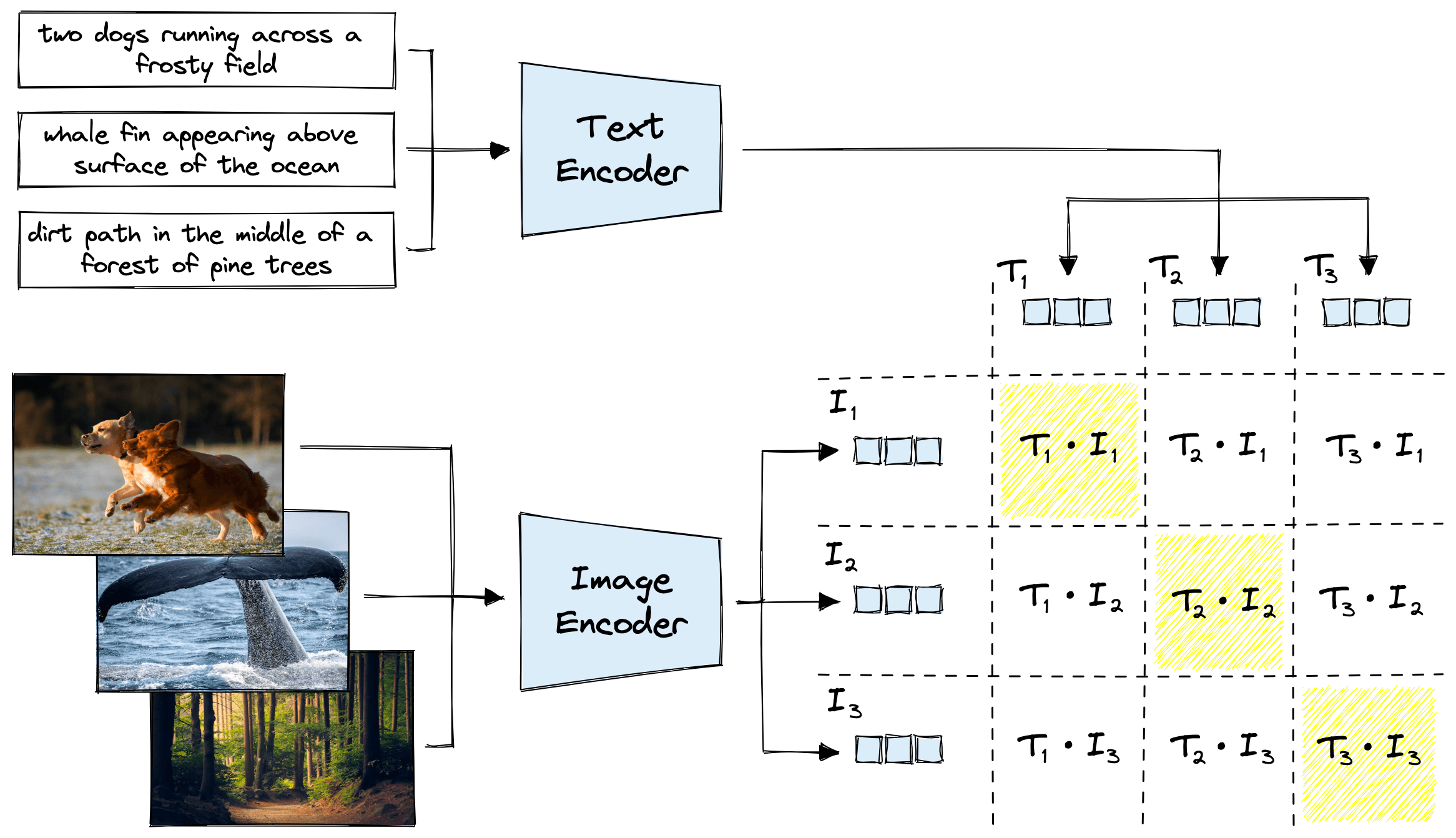
- Calculate Similarity: The model computes the cosine similarity between every possible image embedding and text embedding. This is done by taking the dot product of the (normalized) embedding vectors. This results in an \(N\times N\) similarity matrix. $$
\text{similarity_matrix}[i, j] = \text{cosine_similarity}(I_i, T_j)
$$ - The Contrastive Objective:
- The diagonal of this matrix (\([I_1, T_1]\), \([I_2, T_2]\), etc.) represents the scores for the correct pairs. The off-diagonal elements represent the scores for the \(N\times (N-1)\) incorrect pairs.
This is formulated as a cross-entropy loss. For each image, the model tries to predict which of the \(N\) text descriptions is the correct one. It does this again for each text, predicting the correct image. The total loss is a symmetric cross-entropy loss over these two prediction tasks.
The Power of Zero-Shot Classification
The true power of CLIP is unlocked after training. Because it has learned a general-purpose mapping between visual and textual concepts, it can perform tasks it was never explicitly trained on. The most prominent example is zero-shot image classification.
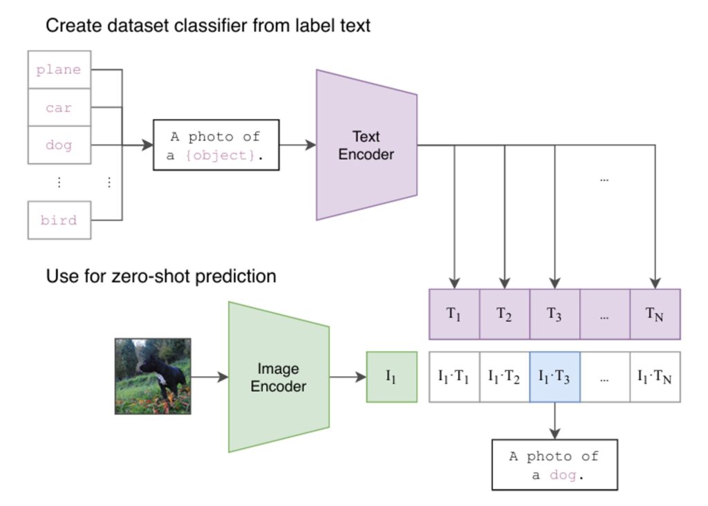
Here is how it works:
- Define Classes: You want to classify an image into one of several categories, for example, “a plane,” “a car,” or “a dog.”
- Create Text Prompts: You turn these categories into descriptive prompts, like “a photo of a plane,” “a photo of a car,” and “a photo of a dog.”
- Embed Everything:
- You pass the image you want to classify through the Image Encoder to get its embedding.
- You pass all your text prompts through the Text Encoder to get a set of text embeddings.
- Compare and Classify: You calculate the cosine similarity between the image embedding and each of the text embeddings. The text prompt that results in the highest similarity is your predicted class.
This is “zero-shot” because the model can classify images into categories it has never seen during its training, simply by being given a textual description of that category.
Code Examples
Zero‑Shot Classification Example
Here is a simple Python snippet showing how to use a pre-trained CLIP model from the transformers library for zero-shot classification.
from PIL import Image
import requests
from transformers import CLIPProcessor, CLIPModel

# Load the pre-trained model and processor
model = CLIPModel.from_pretrained("openai/clip-vit-base-patch32")
processor = CLIPProcessor.from_pretrained("openai/clip-vit-base-patch32")

# Load an image from a URL
url = "http://images.cocodataset.org/val2017/000000039769.jpg" # An image of two cats
image = Image.open(requests.get(url, stream=True).raw)

# Define the candidate labels
candidate_labels = ["a photo of a cat", "a photo of a dog", "a photo of a bird"]

# Process the image and text
inputs = processor(text=candidate_labels, images=image, return_tensors="pt", padding=True)

# Get the model outputs
outputs = model(**inputs)

# The logits_per_image are the similarity scores between the image and each text label
logits_per_image = outputs.logits_per_image

# We apply a softmax to get probabilities
probs = logits_per_image.softmax(dim=1)

# Print the results
for label, prob in zip(candidate_labels, probs[0]):
    print(f"{label}: {prob.item():.4f}")

# Expected Output:
# a photo of a cat: 0.99...
# a photo of a dog: 0.00...
# a photo of a bird: 0.00...Getting Raw Embeddings (For Retrieval)
from datasets import load_dataset
import torch.nn.functional as F
import torch
from PIL import Image, UnidentifiedImageError # Import Image and UnidentifiedImageError for handling image data
import requests # Import requests to fetch images from URLs

# Define the device
device = "cuda" if torch.cuda.is_available() else "cpu"

# Load the conceptual_captions dataset again to ensure it's available in this cell's scope
try:
    data = load_dataset("conceptual_captions", split="train")
    print("Conceptual Captions dataset loaded successfully.")
    # Print the keys of the dataset to inspect its structure
    print("Dataset keys:", data.features.keys())
except Exception as e:
    print(f"Error loading conceptual_captions: {e}")
    # Exit if the dataset couldn't be loaded
    exit()


text_batch = ["a photo of a cat", "a photo of a dog"]
text_inputs = processor(text=text_batch, return_tensors='pt', padding=True).to(device)
with torch.no_grad():
    text_vecs = model.get_text_features(text_inputs['input_ids'], attention_mask=text_inputs['attention_mask'])
text_vecs = F.normalize(text_vecs, p=2, dim=-1)

# Access the image data using key 'image_url' and load the images, skipping invalid ones
image_urls = data[:4]['image_url']
image_batch = []
for url in image_urls:
    try:
        image = Image.open(requests.get(url, stream=True).raw)
        image_batch.append(image)
    except UnidentifiedImageError:
        print(f"Could not identify image from URL: {url}. Skipping.")
    except Exception as e:
        print(f"An unexpected error occurred loading image from URL {url}: {e}. Skipping.")

# Only proceed if there are valid images in the batch
if image_batch:
    image_inputs = processor(images=image_batch, return_tensors='pt').to(device)
    with torch.no_grad():
        image_vecs = model.get_image_features(image_inputs['pixel_values'])
    image_vecs = F.normalize(image_vecs, p=2, dim=-1)

    similarity = image_vecs @ text_vecs.T
    print(similarity)
else:
print("No valid images were loaded from the provided URLs.")Simple Text→Image Retrieval
# Define the query text for retrieval
query = "a dog"

# Tokenize and encode the query text, move to the correct device
q_inputs = processor(text=[query], return_tensors='pt').to(device)

# Generate the text embedding for the query using the CLIP text encoder
with torch.no_grad():
    q_vec = model.get_text_features(q_inputs['input_ids'], attention_mask=q_inputs['attention_mask'])

# Normalize the query embedding to unit length for cosine similarity
q_vec = q_vec / q_vec.norm(dim=-1, keepdim=True)

# Compute similarity scores between each image embedding and the query embedding
scores = (image_vecs @ q_vec.T).squeeze()

# Find the index of the image with the highest similarity score (best match)
best = scores.argmax().item()

# Display the best matching image
print("Best match index:", best)
image_batch[best].show()Educational Patch‑Based Localization (Toy)
import torch, numpy as np, matplotlib.pyplot as plt
from transformers import CLIPProcessor, CLIPModel
from PIL import Image

# Function to split an image into non-overlapping square patches
def create_patches(img, size):
    w, h = img.size
    patches, coords = [], []
    for y in range(0, h, size):
        for x in range(0, w, size):
            patches.append(img.crop((x, y, x+size, y+size)))
            coords.append((x, y))
    return patches, coords, w, h

# Load the CLIP model and processor
model_id = "openai/clip-vit-base-patch32"
processor = CLIPProcessor.from_pretrained(model_id)
model = CLIPModel.from_pretrained(model_id)
device = 'cuda' if torch.cuda.is_available() else 'cpu'
model.to(device)

# Load an example image from a URL
url = "http://images.cocodataset.org/val2017/000000039769.jpg" # An image of two cats
image = Image.open(requests.get(url, stream=True).raw)

# Split the image into patches of size 64x64 pixels
patch_size = 64
patches, coords, W, H = create_patches(image, patch_size)

# Encode all patches using CLIP's image encoder
inputs = processor(images=patches, return_tensors='pt').to(device)
with torch.no_grad():
    patch_vecs = model.get_image_features(inputs['pixel_values'])
patch_vecs = patch_vecs / patch_vecs.norm(dim=-1, keepdim=True) # Normalize for cosine similarity

# Encode the text prompt using CLIP's text encoder
text = "a fluffy cat"
t_inputs = processor(text=[text], return_tensors='pt').to(device)
with torch.no_grad():
    t_vec = model.get_text_features(t_inputs['input_ids'], attention_mask=t_inputs['attention_mask'])
t_vec = t_vec / t_vec.norm(dim=-1, keepdim=True) # Normalize for cosine similarity

# Compute similarity scores between each patch and the text prompt
scores = (patch_vecs @ t_vec.T).squeeze().cpu().tolist()

# Reshape scores into a 2D heatmap matching the patch grid
cols = (W + patch_size - 1) // patch_size
rows = (H + patch_size - 1) // patch_size
heat = np.array(scores).reshape(rows, cols)

# Visualize the heatmap: brighter areas indicate higher relevance to the prompt
plt.imshow(heat, cmap='magma')
plt.title(f"Approx relevance: {text}")
plt.colorbar(); plt.show()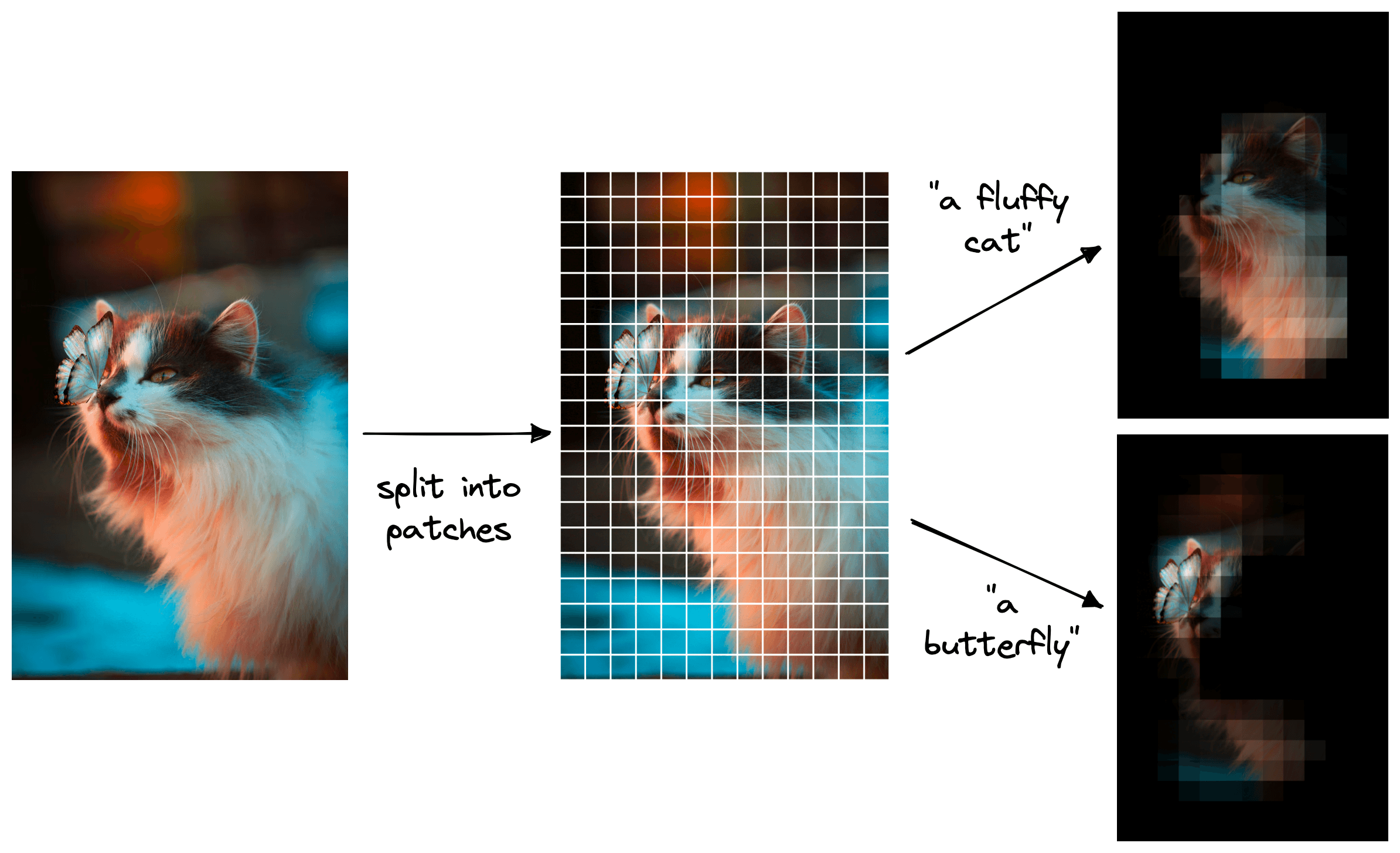
A key application of zero-shot CLIP is object detection, which bypasses the need for traditional bounding-box training. By splitting an image into small patches and comparing the vector embedding of each patch to the vector embedding of a natural language prompt (e.g., “a fluffy cat”), we can generate a heatmap showing the object’s position. This means you can identify an object, such as a cat or a butterfly in a mixed image, just by typing what you’re looking for.
Miscellaneous Details of CLIP
- Dataset Creation: WebImageText (WIT)
To train CLIP, OpenAI curated WIT, a dataset of 400 million image-text pairs sourced from publicly available internet data. Key steps included:- Query-Based Collection: Images were gathered using 500,000 text queries to ensure diversity.
- Balanced Sampling: Up to 20,000 pairs per query prevented overrepresentation of common terms.
- Filtering: Low-quality or non-English content was excluded.
- Training Process
- Optimization: Adam with weight decay and cosine learning rate scheduling.
- Batch Size: 32,768 for efficient contrastive learning.
- Efficiency: Mixed-precision training and gradient checkpointing reduced memory usage.
- Compute: Largest models trained on 592 V100 GPUs for up to 18 days.
- Prompt Engineering and Ensembling
- Contextual Prompts: Adding phrases like “a type of pet” improves accuracy by specifying domain context.
- Ensembling: Combining multiple prompts (e.g., “a small {label}” and “a large {label}”) boosts performance by 3–5%.
- Zero-Shot vs. Supervised Models
- ImageNet: CLIP achieves 76.2% zero-shot accuracy, matching the original ResNet-50 trained on 1.28M labeled images.
- 27-Dataset Benchmark: CLIP outperforms supervised models on 16/27 tasks, including action recognition (Kinetics700) and OCR (Rendered SST2).
- Robustness to Distribution Shifts:
CLIP excels under natural distribution shifts (e.g., adversarial examples, style changes):- Effective Robustness: Reduces the accuracy gap between in-distribution and out-of-distribution data by up to 75%.
- Example: CLIP maintains high accuracy on ImageNet variants (e.g., ImageNet-R, ImageNet Sketch) where traditional models falter.
- Few-Shot Learning
- Data Efficiency: Zero-shot CLIP matches 4-shot linear classifiers and rivals 16-shot models like BiT-M ResNet-152×2.
- Limitation: Performance plateaus when adapting to ImageNet, suggesting overfitting to narrow supervision.
Limitations and Considerations
- Biases in Training Data: Since CLIP is trained on internet data, it may inherit and amplify societal biases present in that data. Care should be taken when deploying CLIP in sensitive applications.
- Interpretability: While CLIP can provide similarity scores, understanding why it made a particular decision can be challenging. Further research into interpretability methods for multi-modal models is ongoing.
- Poor performance on fine-grained classification: CLIP may struggle to distinguish between very similar categories, such as different car models, aircraft variants, or flower species.
- Resolution Limitations: The image encoder may have limitations in handling very high-resolution images, which could affect performance in certain applications.
- Domain Adaptation: CLIP may struggle with images or concepts that are very different from those present in its training data. Fine-tuning on domain-specific data may be necessary for optimal performance.
- Sensitivity to wording or phrasing: Natural language can be ambiguous, and CLIP’s performance may degrade when prompts are vague or context-dependent.
- Limited Context Understanding: CLIP may struggle with understanding the broader context of an image or text, leading to potential misinterpretations.
Applications
- Image Classification: CLIP can classify images into 1000 ImageNet classes.
- Object Detection: CLIP can detect objects in images.
- Visual Question Answering: CLIP can answer questions about images.
- Semantic Image Search and Retrieval: Input natural language queries, and the CLIP model retrieves images that best match the textual descriptions.
- Data Content Moderation: CLIP can assist in the content moderation process by detecting and flagging such content based on natural language criteria.
- Deciphering Blurred Images: CLIP can provide valuable insights by interpreting the available visual information in conjunction with relevant textual descriptions.
- Image Captioning: CLIP can generate captions for images.
- Visual Reasoning: CLIP can perform visual reasoning tasks.
- Visual Dialog: CLIP can engage in dialogues about images.
- Visual Concept Learning: CLIP can learn new visual concepts from textual descriptions.
- Visual Semantic Segmentation: CLIP can segment images into semantic regions.
- Visual Relationship Detection: CLIP can detect relationships between objects in images.
- Geolocation: Predicting locations from satellite imagery using prompts like “a satellite photo of {country}.”
Conclusion
CLIP represents a significant step forward in building AI that understands the world in a more holistic and human-like way. By leveraging vast amounts of unlabeled data from the web and using a simple yet powerful contrastive learning objective, it creates a unified embedding space for text and images. This not only enables remarkable zero-shot capabilities but also provides a foundational building block for a new generation of multi-modal AI systems, from text-to-image generators like DALL-E to more advanced visual reasoning models.

Happy is a seasoned ML professional with over 15 years of experience. His expertise spans various domains, including Computer Vision, Natural Language Processing (NLP), and Time Series analysis. He holds a PhD in Machine Learning from IIT Kharagpur and has furthered his research with postdoctoral experience at INRIA-Sophia Antipolis, France. Happy has a proven track record of delivering impactful ML solutions to clients.
Subscribe to our newsletter!