Machine Learning is often described as “data + algorithms”, but mathematics is the glue that makes everything work.
At its core, ML is about:
Modeling uncertainty, learning from data, and making optimal decisions.
Machine Learning can look like “just code”, but most algorithms are careful combinations of:
- Probability (to represent uncertainty)
- Information theory (to measure surprise/error)
- Estimation (to choose parameters)
- Optimization (to actually find those parameters)
- Latent-variable methods (when something is hidden)
- Stochastic processes (for sequences and sampling)
This note is a connected roadmap. It starts with the high-level map (what connects to what), then drills into the minimal technical pieces you actually use.
1. The Concept Map
1.1 The big picture
Most of machine learning boils down to distribution matching.
Imagine two curves:
- The Reality ($P$): The true, messy distribution of data in the real world (e.g., the actual probability that an image contains a cat). We never see this fully; we only see samples (our dataset).
- The Model ($Q_\theta$): The simplified curve our model draws, controlled by knobs and dials called parameters ($\theta$).
Learning is simply the process of twisting the knobs ($\theta$) until our model’s curve ($Q_\theta$) looks as much like reality ($P$) as possible.
- To measure “how different” $P$ and $Q$ are, we use KL-Divergence.
- In practice, this simplifies to minimizing Cross-Entropy (for classification) or maximizing Likelihood.
- If we add a penalty to accurate weights, we are doing MAP (Bayesian inference).
Probability & Bayesian modeling
- Random variables, distributions (Bernoulli, Categorical, Gaussian)
- Conditional probability and the product rule
- Bayes’ theorem: The rule for updating beliefs based on new evidence.
- Prior (before seeing data)
- Likelihood (how well parameters explain data)
- Evidence (normalizing constant)
- Posterior (updated belief after seeing data)
- Posterior predictive (predictions after learning)
Information theory
- Self-information $I(x)=-\log p(x)$: A measure of “surprise” for an event $x$ with probability $p(x)$.
- Entropy $H(P)$: A measure of uncertainty, randomness, or “surprise” in a probability distribution $P$.
- Cross-entropy $H(P,Q)$: The expected surprise when events from distribution $P$ are encoded using a code optimized for distribution $Q$.
- KL-divergence $D_{\mathrm{KL}}(P|Q)$ : A way to measure the difference between two probability distributions (e.g., true data vs. our model).
- Information gain (reduction in entropy)
Parameter estimation
- Likelihood and log-likelihood: Measures of how well model parameters explain observed data.
- Maximum Likelihood Estimation (MLE): A method to find the model parameters that make the observed data most likely.
- Maximum a Posteriori (MAP): an extension of MLE that incorporates a prior (closely related to regularization).
- Regularization as priors (L2 ↔ Gaussian, L1 ↔ Laplace)
Optimization (how parameters are found)
- Gradients and (stochastic) gradient descent: basic tool for optimizing parameters
- Loss landscapes (why optimization is hard)
- Convexity (why some problems are easier)
- Newton / quasi-Newton (why curvature of log-likelihood matters)
Latent variables & incomplete data
- Latent variables (hidden cluster label, topic assignment, hidden state): variables that affect observations but are not directly observed
- Jensen’s inequality: allows lower-bounding complex objectives
- Expectation-Maximization (EM): An iterative algorithm to find parameters when some data is missing or hidden (Latent Variables).
Sequences & stochastic processes
- Markov chains: A stochastic model describing a sequence of possible events where the probability of each event depends only on the state attained in the previous event.
- Stationary distribution and mixing
- Hidden Markov Models (HMMs)
- MCMC (Markov chains for sampling complex posteriors): building a Markov chain whose stationary distribution is the target posterior distribution.
You can think of ML as probability + optimization + information theory working together.
2. Probability foundations you actually use
ML models do not give certainties — they give probabilities (and, during training, likelihoods).
Examples:
- “There is a 90% chance this email is spam” (a predicted probability)
- “This image is most likely a cat” (the highest-probability class)
To work with uncertainty, we need the language of probability.
- Random Variable: A quantity whose value depends on chance (e.g., class label)
- Probability Distribution: Describes how likely each value is
Probability is the foundation for Bayes, MLE, MAP, EM, and Markov models.
2.1 Conditional probability and the product rule
The product rule is the basic identity that lets probability “factor” complex events:
$$P(A,B)=P(A\mid B)P(B)=P(B\mid A)P(A).$$
In ML, this shows up whenever you rewrite joint probabilities into things you can model.
2.2 Bayes’ theorem: prior → posterior
Bayes’ theorem is just the product rule rearranged:
$$P(\theta\mid D)=\frac{P(D\mid \theta)\,P(\theta)}{P(D)}.$$
Interpretation:
- Prior $P(\theta)$: belief about parameters before seeing data
- Likelihood $P(D\mid\theta)$: how well $\theta$ explains the observed data
- Posterior $P(\theta\mid D)$: updated belief after data
- Evidence $P(D)$: normalizer that makes the posterior a valid distribution
Connections:
- This framework is the foundation for MAP estimation: pick parameters that are likely under both the data (likelihood) and your prior.
- MCMC becomes useful when $P(\theta\mid D)$ is hard to compute analytically.
- Many regularizers correspond to choosing a prior $P(\theta)$.
2.3 Law of Large Numbers & Central Limit Theorem
Law of Large Numbers (LLN): averaging stabilizes estimates
Treat each sample as a noisy measurement. Averaging many samples cancels noise.
Let $X_1,X_2,\dots$ be i.i.d. with mean $\mu=\mathbb{E}[X_i]$ (and finite variance). The sample mean is
$$\bar X_n=\frac{1}{n}\sum_{i=1}^n X_i.$$
Weak LLN: for any $\varepsilon>0$,
$$\Pr\left(|\bar X_n-\mu|>\varepsilon\right)\to 0\quad\text{as }n\to\infty.$$
Practical ML connection:
- Empirical risk minimization relies on LLN: the average training loss approaches the true expected loss under the data distribution.
- Mini-batch gradients are noisy estimates of the full gradient; averaging over more samples reduces variance.
Central Limit Theorem (CLT): fluctuations look Gaussian
LLN says $\bar X_n$ converges to $\mu$. CLT describes the shape of the error around $\mu$.
If $X_1,\dots,X_n$ are i.i.d. with variance $\sigma^2\in(0,\infty)$, then
$$\frac{\sqrt{n}(\bar X_n-\mu)}{\sigma}\;\overset{d}{\Rightarrow}\;\mathcal{N}(0,1),$$
so for large $n$,
$$\bar X_n\approx \mathcal{N}\left(\mu,\;\frac{\sigma^2}{n}\right).$$
Practical ML connection:
- Uncertainty estimates for averages: standard errors scale like $\sigma/\sqrt{n}$.
- A/B testing and offline evaluation: many test statistics are approximately normal by CLT.
- Why Gaussian noise models work: aggregating many small independent effects often yields something close to normal.
3. Information theory: entropy, cross-entropy, KL-divergence
To learn from data, we need a way to quantify information and error.
3.1 Self-information (surprise)
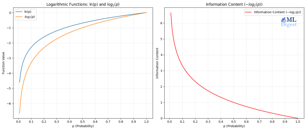
If an outcome has probability $p(x)$, its “surprise” is:
$$I(x)=-\log p(x).$$
Rare events ($p(x)$ small) have large surprise.
3.2 Entropy (uncertainty of a distribution)
Entropy (Shannon Entropy) measures the average level of “uncertainty” or “surprise” inherent to a variable’s possible outcomes.
For a discrete distribution $P$ over outcomes $x$:
$$H(P)=\mathbb{E}_{x\sim P}[-\log P(x)] = -\sum_x P(x)\log P(x).$$
Intuition:
- High entropy: outcomes are spread out / unpredictable (e.g., a fair coin flip: 50/50).
- Low entropy: one outcome dominates / predictable (e.g., a loaded coin that is always Heads)
Where it appears:
- Decision trees choose splits that reduce entropy (increase information gain).
3.3 KL-divergence (gap between $P$ and $Q$)
Kullback-Leibler (KL) Divergence measures how one probability distribution diverges from a reference distribution. It is often used like a “distance”, but it is not a true metric.
$$D_{\mathrm{KL}}(P|Q)=\mathbb{E}_{x\sim P}\left[\log \frac{P(x)}{Q(x)}\right].$$
Key facts:
- $D_{\mathrm{KL}}(P|Q)\ge 0$, and equals $0$ iff $P=Q$ (almost everywhere)
- It is not symmetric: $D_{\mathrm{KL}}(P|Q)\ne D_{\mathrm{KL}}(Q|P)$
A practical caveat: $D_{\mathrm{KL}}(P|Q)$ is finite only when $Q(x)>0$ wherever $P(x)>0$ (support mismatch can make the KL infinite). In standard classification, softmax outputs strictly positive probabilities, which typically avoids this pitfall.
3.4 Cross-entropy (expected surprise under the model)
If the world follows $P$ but your model uses $Q$:
$$H(P,Q)=\mathbb{E}_{x\sim P}[-\log Q(x)].$$
This is the expected surprise you would experience if you “bet” using $Q$.
$$H(P,Q)=H(P)+D_{\mathrm{KL}}(P|Q).$$
Since $H(P)$ does not depend on your model parameters $\theta$, minimizing cross-entropy over $Q_\theta$ is equivalent to minimizing $D_{\mathrm{KL}}(P|Q_\theta)$. Thus,
- Cross-entropy = entropy + KL-divergence
- Minimizing cross-entropy ≈ minimizing KL-divergence
Where it appears:
- Cross-entropy is the basis for classification losses (e.g., log loss for logistic regression, softmax cross-entropy for multi-class).
Cross-entropy → KL → MLE (a tiny worked example)
Consider a classification dataset $(x_i, y_i)$ with one-hot labels and a model $Q_\theta(y\mid x)$. The empirical cross-entropy is
$$\hat H(P, Q_\theta) = -\frac{1}{n} \sum_{i=1}^n \log Q_\theta(y_i\mid x_i).$$
This is exactly the negative log-likelihood (up to the $1/n$ factor), so minimizing cross-entropy is equivalent to maximum likelihood estimation for conditional models.
4. Likelihood and Maximum Likelihood Estimation (MLE)
Suppose you have data $D={x_1,\dots,x_n}$ and a parametric model $P(x\mid\theta)$.
4.1 Likelihood
The likelihood is the probability (density, for continuous variables) of the data under parameters $\theta$:
$$\mathcal{L}(\theta)=P(D\mid\theta).$$
With the common i.i.d. assumption (data points are independent and identically distributed):
$$P(D\mid\theta)=\prod_{i=1}^n P(x_i\mid\theta).$$
4.2 Log-likelihood
We almost always optimize the log-likelihood:
$$\ell(\theta)=\log \mathcal{L}(\theta)=\sum_{i=1}^n \log P(x_i\mid\theta).$$
Why logs:
- products become sums (easier calculus)
- better numerical stability
4.3 MLE definition
$$\hat\theta_{\mathrm{MLE}} = \arg\max_\theta \log P(D\mid\theta).$$
Connections:
- Minimizing negative log-likelihood is a standard training loss.
- In common cases, MLE recovers familiar objectives:
- Linear regression + Gaussian noise → squared error
- Logistic regression + Bernoulli → cross-entropy / log loss
5. Maximum a Posteriori (MAP): MLE + prior
5.1 Definition
MAP maximizes the posterior instead of only the likelihood:
$$\hat\theta_{\mathrm{MAP}} = \arg\max_\theta P(\theta\mid D)
=\arg\max_\theta P(D\mid\theta)P(\theta).$$
Taking logs:
$$\hat\theta_{\mathrm{MAP}} = \arg\max_\theta \left[\log P(D\mid\theta)+\log P(\theta)\right].$$
So MAP = “fit the data” + “prefer certain parameters”.
5.2 Regularization as a prior
If your training objective looks like:
$$\min_\theta \left( -\log P(D\mid\theta) + \lambda\,\Omega(\theta) \right),$$
it often corresponds to a prior of the form $P(\theta)\propto e^{-\lambda\Omega(\theta)}$.
Common correspondences:
- L2 regularization $\Omega(\theta)=|\theta|_2^2$ ↔ Gaussian prior (weights near 0)
- L1 regularization $\Omega(\theta)=|\theta|_1$ ↔ Laplace prior (sparsity)
5.3 MLE vs. MAP (what changes in practice)
How do we choose the “best” parameters (weights) for our model? We usually use one of these two approaches. The table below summarizes the key differences:
| Aspect | Maximum Likelihood Estimation (MLE) | Maximum a Posteriori (MAP) |
|---|---|---|
| Core Question | What parameters make my observed data most probable? | What parameters are most probable given the data AND my prior beliefs? |
| Formula | $\hat\theta_{\mathrm{MLE}} = \arg\max_\theta P(D\mid\theta)$ | $\hat\theta_{\mathrm{MAP}} = \arg\max_\theta P(D\mid\theta)P(\theta)$ |
| Prior Knowledge | Does not use prior information about parameters | Incorporates prior beliefs about parameters ($P(\theta)$) |
| Interpretation | Focuses only on fitting the observed data | Balances fit to data with preference for certain parameter values |
| Example | In Linear Regression, minimizing the Sum of Squared Errors (Least Squares) is the MLE under Gaussian noise | Adding L2 regularization (Ridge) is equivalent to MAP with a Gaussian prior |
Summary:
- MLE looks solely at the data, maximizing the likelihood function $L(\theta)$.
- MAP augments MLE by multiplying the likelihood by a prior probability $P(\theta)$, thus incorporating prior beliefs.
Many ML models include latent variables $Z$ you do not observe (cluster IDs, hidden states, mixture component selection).
If you observed $(X,Z)$, MLE/MAP may be easy. But you only observe $X$.
6.1 The core difficulty: marginal likelihood
You want to maximize:
$$\log P(X\mid\theta)=\log \sum_Z P(X,Z\mid\theta).$$
The $\log\sum$ structure is what makes direct optimization hard.
6.2 The EM algorithm
EM alternates two steps:
- E-step (Expectation): compute the posterior over latent variables under current parameters
$$q(Z) \leftarrow P(Z\mid X,\theta^{(t)}).$$ - M-step (Maximization): update parameters to maximize the expected complete-data log-likelihood
$$\theta^{(t+1)} \leftarrow \arg\max_\theta \mathbb{E}_{Z\sim q}[\log P(X,Z\mid\theta)].$$
The Algorithm:
- E-Step (Expectation): Guess the missing/hidden values based on current parameters (calculate probabilities).
- M-Step (Maximization): Update the parameters to maximize likelihood, assuming the guesses from the E-step were correct.
- Repeat until convergence.
6.3 Connections and examples
- GMMs: E-step produces responsibilities; M-step updates means/covariances
- HMMs: EM becomes Baum–Welch
- k-means: a limiting/special case of EM with hard assignments
Deeper connection:
- EM can be derived using Jensen’s inequality and a lower bound called the ELBO (tight when $q(Z)=P(Z\mid X,\theta)$).
- Variational inference generalizes the E-step idea by constraining $q(Z)$ to a simpler family.
7. Markov chains: sequences and sampling
7.1 Markov property
A Markov Chain is a mathematical system that undergoes transitions from one state to another according to certain probabilistic rules. The defining characteristic is the Markov Property (Memorylessness):
“The future depends only on the present, not on the past.”
$$ P(X_{t+1} | X_t, X_{t-1}, …) = P(X_{t+1} | X_t) $$
So the future depends only on the present.
Connections to ML
- N-grams: simplified language model via Markov assumptions
- HMMs: latent state sequence is a Markov chain; observations depend on states
- Reinforcement learning: Markov Decision Processes (MDPs) extend Markov chains with actions and rewards
- MCMC (Markov Chain Monte Carlo): build a Markov chain whose stationary distribution is the posterior $P(\theta\mid D)$
8. How these concepts connect in practice (quick recipes)
8.1 Probabilistic classification
- Model a conditional distribution $Q_\theta(y\mid x)$.
- Train via negative log-likelihood:
$$\min_\theta -\sum_i \log Q_\theta(y_i\mid x_i).$$ - This is cross-entropy; minimizing it is minimizing a KL to the true label distribution.
- Add L2 regularization → becomes MAP with a Gaussian prior.
8.2 Decision trees
- Choose splits that reduce entropy of labels.
- “Information gain” is an information-theoretic measure of improved purity.
8.3 Mixture models / clustering
- Hidden variable: which component generated a point.
- Fit with EM by alternating soft assignments and parameter updates.
- Add priors → EM-style MAP updates (semi-Bayesian mixture modeling).
8.4 Bayesian inference
- Bayes gives the posterior.
- When integrals are hard, use:
- MCMC (samples via Markov chains)
- Variational inference (optimize an ELBO, often involving KL terms)
9. Cheat sheet of key equations
- Bayes: Posterior $\propto$ Likelihood $\times$ Prior
$$P(\theta\mid D)=\frac{P(D\mid\theta)P(\theta)}{P(D)}$$ - Entropy: Average uncertainty
$$H(P)=-\sum_x P(x)\log P(x)$$ - Cross-entropy: Expected surprise of model $Q$ on data $P$
$$H(P,Q)=\mathbb{E}_{x\sim P}[-\log Q(x)]$$ - KL divergence: Distance between distributions
$$D_{\mathrm{KL}}(P|Q)=\mathbb{E}_{x\sim P}\left[\log\frac{P(x)}{Q(x)}\right]$$ - Relationship:
$$H(P,Q)=H(P)+D_{\mathrm{KL}}(P|Q)$$ - MLE: Fit data perfectly
$$\hat\theta_{\mathrm{MLE}}=\arg\max_\theta \log P(D\mid\theta)$$ - MAP: Fit data + Keep parameters reasonable
$$\hat\theta_{\mathrm{MAP}}=\arg\max_\theta [\log P(D\mid\theta)+\log P(\theta)]$$ - Markov property:
$$P(X_{t+1}\mid X_t,\dots)=P(X_{t+1}\mid X_t)$$
10. If you only remember five connections
- Cross-entropy is expected surprise under your model $Q$.
- Minimizing cross-entropy is minimizing KL divergence to the true distribution.
- Minimizing that KL (in standard supervised setups) is equivalent to maximizing likelihood (MLE).
- Adding regularization is often MAP: MLE + log prior.
- With hidden variables, EM is a classic likelihood-based method; and when posteriors are hard to integrate, MCMC uses Markov chains to sample.

Silpa brings 5 years of experience in working on diverse ML projects, specializing in designing end-to-end ML systems tailored for real-time applications. Her background in statistics (Bachelor of Technology) provides a strong foundation for her work in the field. Silpa is also the driving force behind the development of the content you find on this site.
Subscribe to our newsletter!