Imagine you are reading a mystery novel. The clue you find on page 10 is crucial for understanding the twist on page 12. But the description of the weather on page 1? Probably less so. As you read, your attention naturally prioritizes recent information while keeping a faded memory of what happened earlier.
In Transformer models, understanding this order — and the distance between words — is crucial. A sentence like “The dog chased the cat” means something entirely different from “The cat chased the dog.” The mechanism that helps models understand this order is called positional encoding.
For a long time, many architectures used methods that added positional information directly to the word embeddings. You can think of this as giving each word a “GPS coordinate” (for example, “Word #5”) before it enters the model. While effective, these methods had a significant limitation: they struggled when a sentence was longer than any sentence they had seen during training. This is known as the extrapolation problem. If a model was trained on 500‑word essays, it can be completely lost trying to read a 2,000‑word chapter.
ALiBi, which stands for Attention with Linear Biases, offers an elegant and surprisingly simple solution to this problem. It was introduced in the paper “Train Short, Test Long: Attention with Linear Biases Enables Input Length Extrapolation”. At a high level, ALiBi bakes a very simple assumption into the attention mechanism: recent tokens matter more than distant ones, but different heads should decay at different rates.
If you are familiar with RoPE (Rotary Position Embeddings), you can think of ALiBi as taking the opposite route: instead of encoding position by rotating the \(Q\) and \(K\) vectors themselves, it leaves the content vectors unchanged and directly shapes the attention logits with a simple distance‑based bias. A more detailed comparison appears in the section “Comparison with RoPE” below.
Intuition: The “Proximity Bias”
Instead of adding positional information to the word embeddings, ALiBi introduces a proximity bias directly into the attention mechanism.
Imagine you are in a conversation. You naturally pay more attention to the words someone has just said compared to words they said five minutes ago. The recency of the information creates a bias in your attention. ALiBi works on a similar principle. It tells the attention mechanism that words closer to each other are likely more relevant to each other.
It achieves this by adding a small “penalty” to the attention score between two words based on how far apart they are. The further apart the words, the larger the penalty, and the less attention they will pay to each other.
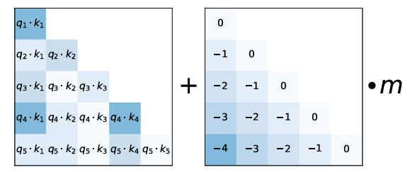
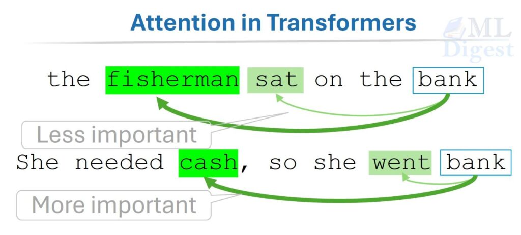
In the visualization above, observe how this penalty is applied. On the left, you have the standard attention scores (the dot product of Query and Key). On the right, ALiBi subtracts a value based on the distance.
Think of this as applying a mask of varying transparency over the text history. For recent words, the mask is clear. As you look further back, the mask becomes more opaque, making it harder for the model to “see” or attend to those words.
Crucially, ALiBi uses a different “fading rate” or slope for each attention head. This is the secret sauce that allows it to balance local and global context:
- The Magnifying Glass (Steep Slope): Some heads have a very steep penalty. They focus intensely on the immediate neighbors—the last few words. These heads are excellent for understanding local grammar, such as knowing that “the” is usually followed by a noun.
- The Telescope (Gentle Slope): Other heads have a very gentle penalty. They can look far back into the context with almost no degradation. These heads capture long-range dependencies, such as a character name mentioned chapters ago.
This variety allows the model to capture both the immediate syntactic structure and the broad narrative arc simultaneously.
Rigor: the technical details
The core of the Transformer’s attention mechanism is the scaled dot-product attention formula:
$$
\text{Attention}(Q, K, V) = \text{softmax}\left(\frac{QK^T}{\sqrt{d_k}}\right)V
$$
Here, \(Q\) (Query), \(K\) (Key), and \(V\) (Value) are matrices representing the words in the sequence. The \(QK^T\) operation calculates the attention scores between every pair of words.
ALiBi modifies this by adding a static, non‑learned bias matrix directly to the \(QK^T\) term before the softmax operation.
$$
\text{Attention}(Q, K, V) = \text{softmax}\left(\frac{QK^T}{\sqrt{d_k}} + \text{bias}\right)V
$$
The key design choice is how this \(\text{bias}\) matrix is constructed. For an attention head \(h\), the bias added to the attention score between query \(i\) (the current position) and key \(j\) (a past position) is:
$$
\text{bias}_{ij}^{(h)} = -m_h \cdot |i – j|
$$
where:
- \(|i – j|\) is the distance between the query token and the key token. Since we usually look at past tokens (\(j \le i\)), this is simply \((i – j)\).
- \(m_h\) is a head-specific scalar (slope) that is fixed and not learned.
The slopes \(m_h\) are not learned parameters; they are fixed geometric sequences. For example, if we have 8 heads, the slopes would be the geometric sequence: \(\frac{1}{2^1}, \frac{1}{2^2}, \dots, \frac{1}{2^8}\).
- Large \(m_h\) (e.g., \(1/2\)): Strong penalty for distance. The head focuses only on very local context.
- Small \(m_h\) (e.g., \(1/256\)): Weak penalty. The head can attend to distant tokens almost as easily as nearby ones.
Because the bias is a simple linear function of the distance, it is called a Linear Bias.
Why Does This Work So Well?
- Excellent extrapolation: Since the bias is a relative measure of distance, it does not matter if a sentence has 100 words or 10,000 words. A distance of 5 is always a distance of 5. The model learns to handle attention based on these relative distances, so the pattern of preferences between “near” and “far” tokens is preserved even when absolute positions become much larger than during training.
- Simplicity and efficiency: ALiBi removes the need for positional embedding layers (such as sinusoidal or learned embeddings). This simplifies the model architecture and eliminates the computational overhead of adding these embeddings at the input layer. The bias is a static value that can be pre‑computed (or computed on the fly) and added during the attention calculation.
- Inductive bias: ALiBi introduces a strong inductive bias — a built‑in assumption — that nearby tokens are more important. This is a very reasonable assumption for most natural language tasks and helps the model learn faster and more effectively. In domains where very long‑range dependencies dominate, this strong locality bias is balanced by the heads with very small slopes.
(Image adapted from the original ALiBi paper)
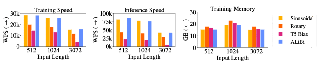
Across batched training, inference speed, and memory use, ALiBi is broadly comparable to sinusoidal, rotary, and T5 bias methods. Speed differences between sinusoidal and ALiBi are negligible and do not meaningfully affect training or inference.

Think of reading a novel that suddenly gets longer: some positional encodings lose the thread as chapters stretch, but ALiBi keeps the narrative coherent. In the above figure, the x‑axis is the validation input length (longer to the right) and the y‑axis is perplexity (lower is better); sinusoidal, rotary, and T5 positional methods show rising perplexity as sequences exceed training lengths, while ALiBi’s curve stays markedly lower and far more stable. This visual comparison highlights ALiBi’s robustness to length extrapolation: by encoding a simple, head‑specific linear distance bias directly in attention, the model preserves low perplexity on longer contexts where other positional schemes fail.
Comparison with RoPE
RoPE (Rotary Position Embeddings) is another popular positional method used in many modern LLMs (such as LLaMA and GPT‑NeoX). While ALiBi and RoPE both aim to make attention aware of token positions and to extrapolate beyond training lengths, they do so in very different ways.
At a high level:
- ALiBi: Modifies the attention scores by adding a head‑specific linear distance penalty. It acts on the interaction between tokens.
- RoPE: Modifies the query and key vectors themselves by rotating them in a complex plane using sinusoidal functions of position. It acts on the representation of the tokens.
Practical Trade‑offs
- Extrapolation: ALiBi tends to extrapolate more gracefully to much longer contexts than seen during training, especially when the model was trained on relatively short sequences. RoPE can extrapolate reasonably well but often benefits from careful rescaling or interpolation tricks when pushing context lengths far beyond training (for example, “NTK scaling” or RoPE interpolation in LLaMA‑style models).
- Implementation Simplicity: ALiBi is extremely simple to implement: it only requires adding a bias term that is a linear function of token distance. RoPE requires implementing the rotary transform on $Q$ and $K$, which is slightly more involved but still efficient in fused kernels.
- Symmetry and Structure: RoPE preserves certain geometric properties (such as rotation invariance within 2D subspaces of the embedding), which some practitioners find beneficial for tasks where relative ordering and periodic patterns matter. ALiBi, by contrast, bakes in a very direct monotonic “closer is better” assumption.
- Adoption in LLM Families: RoPE is used in families such as GPT‑NeoX, LLaMA, ChatGLM, and many derivative models. ALiBi appears in models such as BLOOM, MPT, and StarCoder, especially where long‑context generalization from short‑context training is a first‑class goal.
In practice, both methods are strong choices. ALiBi is appealing when you want robust length extrapolation with minimal architectural changes. RoPE is attractive when you prefer embedding‑level positional structure that integrates smoothly with complex attention kernels and has become a de‑facto default in many LLaMA-derivative families.
Code example: implementing ALiBi in PyTorch
Here is a simplified example of how you might implement the ALiBi bias in a PyTorch‑based attention mechanism.
import torch
import torch.nn as nn
import math

def get_alibi_slopes(num_heads: int) -> torch.Tensor:
    """Return a tensor of slopes for ALiBi.

    This is a simplified version of the logic used in the official implementation.
    For 8 heads, this returns approximately [1/2, 1/4, 1/8, ..., 1/256].
    """
    # We want a geometric sequence where the ratio depends on the number of heads.
    x = (2 ** 8) ** (1 / num_heads)
    slopes = torch.tensor([1 / (x ** (i + 1)) for i in range(num_heads)])
    return slopes.unsqueeze(1).unsqueeze(1)  # Shape: (num_heads, 1, 1)

def build_alibi_bias(seq_len: int, num_heads: int) -> torch.Tensor:
    """Build the ALiBi bias tensor of shape (num_heads, seq_len, seq_len)."""

    # 1. Get the slopes for each head
    slopes = get_alibi_slopes(num_heads)  # (num_heads, 1, 1)

    # 2. Create a relative position matrix
    # positions: [0, 1, 2, ..., seq_len-1]
    positions = torch.arange(seq_len, dtype=torch.float32)

    # relative_positions[i, j] = j - i
    # For causal attention, we care about j <= i, so j - i is negative or zero.
    relative_positions = positions.unsqueeze(0) - positions.unsqueeze(1)  # (1, L) - (L, 1) -> (L, L)

    # 3. Compute the bias
    # We want a penalty, so the bias should be negative.
    # Since relative_positions (j - i) is already negative for the past,
    # we just multiply by the positive slopes.
    # bias = slope * (negative distance)
    alibi_bias = slopes * relative_positions.unsqueeze(0) # (num_heads, seq_len, seq_len)

    # 4. Apply causal mask
    # We strictly mask out the future (where j > i).
    # The ALiBi bias is only relevant for the past (j <= i).
    causal_mask = torch.triu(torch.ones(seq_len, seq_len) * float('-inf'), diagonal=1)

    # Combine them
    final_mask = alibi_bias + causal_mask.unsqueeze(0)

    return final_mask

# --- Usage Example ---
num_heads = 8
seq_len = 10

# Attention scores (dummy data) representing QK^T / sqrt(d_k)
attention_scores = torch.randn(1, num_heads, seq_len, seq_len)

# Get the ALiBi bias
alibi = build_alibi_bias(seq_len, num_heads)

# Add the bias to the attention scores
biased_scores = attention_scores + alibi

# Apply softmax
attention_weights = nn.functional.softmax(biased_scores, dim=-1)

print(f"ALiBi bias shape: {alibi.shape}")
# Check the bias for the first head at the last position
print(f"Bias for Head 0 at last position (looking back 1 step): {alibi[0, -1, -2].item():.4f}")Conclusion
ALiBi is a powerful and intuitive technique that has become a key component in many modern large language models (such as BLOOM and MPT). By replacing absolute positional embeddings with a simple, relative bias in the attention mechanism, it not only solves the critical problem of length extrapolation but also improves model efficiency.
It teaches us a valuable lesson in AI design: sometimes, instead of adding more complex layers or embeddings, the best solution is to bake a strong, sensible assumption (like “recent things matter more”) directly into the mathematics of the model.

Happy is a seasoned ML professional with over 15 years of experience. His expertise spans various domains, including Computer Vision, Natural Language Processing (NLP), and Time Series analysis. He holds a PhD in Machine Learning from IIT Kharagpur and has furthered his research with postdoctoral experience at INRIA-Sophia Antipolis, France. Happy has a proven track record of delivering impactful ML solutions to clients.
Subscribe to our newsletter!