Imagine you are reading a mystery novel, but the pages are torn out and shuffled. You have all the information, but the narrative flow is lost. In the world of Transformers, this is the positional encoding problem: the model processes all tokens simultaneously, so without positional signals it cannot distinguish between “the dog chased the cat” and “the cat chased the dog.”
To solve this, early architectures used Absolute Positional Embeddings. This is like writing a page number on every word. “The” is at position 1, “dog” is at position 2. While this restores order, it is brittle. In human language, the absolute position of a word is rarely significant. It does not matter if the word “therefore” appears at the beginning or the end of a book; what matters is that it connects the premise immediately preceding it to the conclusion immediately following it.
We need a system that emphasizes relative distance. The relationship between a subject and a verb should look the same to the model whether they appear at index 5 and 6, or index 500 and 501. Standard absolute embeddings struggle to represent this invariance efficiently, often failing when sequences grow longer than what the model saw during training.
As models grew in size and complexity, these initial approaches revealed their limitations, especially when faced with the demands of modern LLMs: the need for longer context windows, better generalization to unseen sequence lengths, and efficiency in training and inference. This need for a relative, invariant signal led researchers to look at geometry—specifically, the mathematics of rotation.
Enter Rotary Positional Embeddings (RoPE).
Instead of stamping a number, imagine we treat each word’s embedding vector like a hand on a clock. To encode position, we rotate the vector.
- Position 1: Rotate the vector by 10 degrees.
- Position 2: Rotate the vector by 20 degrees.
- Position 3: Rotate the vector by 30 degrees.
Here is the magic: If you want to know the relationship between the word at Position 1 and the word at Position 3, you do not need to know their absolute angles (10 and 30). You only need to know the difference between them: 20 degrees.
By encoding position as a rotation, RoPE naturally captures the relative distance between tokens. It combines the best of absolute positioning (each token has a unique rotation) and relative positioning (the interaction depends on the angle difference).
RoPE has become a cornerstone of modern LLMs like Llama, Qwen, Gemma, Deepseek, and others.
Why RoPE? The Limitations of Traditional Methods
Positional embeddings (PE) are essential for injecting sequential order information into the otherwise position-agnostic self-attention mechanism. Before we dive into the mechanics of RoPE, let us understand the shortcomings of the methods that preceded it.
- Absolute Positional Embeddings (APE): The original Transformer used fixed sinusoidal functions or learned unique vectors for each absolute position (1st, 2nd, 3rd, etc.). These are added to the token embeddings.
- Pros: Simple to implement and effective for the fixed-length sequences they are trained on.
- Shortcomings:
- Poor Generalization: APE struggles to generalize to sequence lengths not seen during training. If a model is trained on 2048 tokens, its performance degrades significantly when processing 4096 tokens because it has no representation for positions beyond 2048.
- Lack of Relative Understanding: The model does not inherently understand that the relationship between position 5 and 6 is the same as between 105 and 106. It must learn these relationships from scratch for all position pairs, which is data-intensive and inefficient.
- Fixed Representation: The positional representation is a fixed offset, independent of the token itself. This lacks the dynamic, input-dependent nature that could benefit query-key interactions.
- Relative Positional Embeddings (RPE): Later methods tried to directly encode the relative distance between tokens. For example, the model would learn a specific embedding for a distance of “+1” (the next token) and “-2” (two tokens before). These relative embeddings are typically incorporated by adding a learned bias to the attention score matrix based on the distance between tokens.
- Pros: Captures relative positions more naturally, which is a better fit for how language works.
- Shortcomings:
- Computational Inefficiency: RPE often adds complexity and computational overhead to the attention calculation. Modifying the attention matrix directly can be slow and memory-intensive.
- Inference Complexity: These methods can complicate inference, particularly with the Key-Value (KV) cache that is crucial for efficient autoregressive decoding. Storing and accessing relative biases can increase memory usage and latency.
- Limited Flexibility: While better than APE, many RPE implementations are still not as flexible or scalable as needed for the very long context windows of modern LLMs.
RoPE elegantly addresses these issues by encoding relative position information directly into the query and key vectors of the attention mechanism, without adding any trainable parameters or complicating the core attention formula. This makes it highly efficient for both training and inference.
The Mathematics: Rotation is All You Need
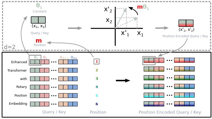
Imagine each word embedding as a vector in a 2D plane. To encode its position, RoPE rotates this vector by an angle that depends on its position in the sequence. For a token at position \(m\), we rotate its embedding by an angle \(m \cdot \theta\). For a token at position \(n\), we rotate it by \(n \cdot \theta\).
Now, how does this help the attention mechanism? The dot product between two vectors is a measure of their similarity. In the attention mechanism, the dot product between a query vector \(q\) and a key vector \(k\) determines the attention score.
If we rotate both the query vector \(q\) (at position \(m\)) and the key vector \(k\) (at position \(n\)) using RoPE, their dot product becomes dependent only on their original embeddings and their relative distance (\(m – n\)). The absolute positions \(m\) and \(n\) magically disappear from the final dot product calculation!
The true elegance of RoPE lies in a fundamental property of rotations: the inner product between two rotated vectors is equivalent to the inner product of the original vectors, but viewed from a rotated frame of reference.
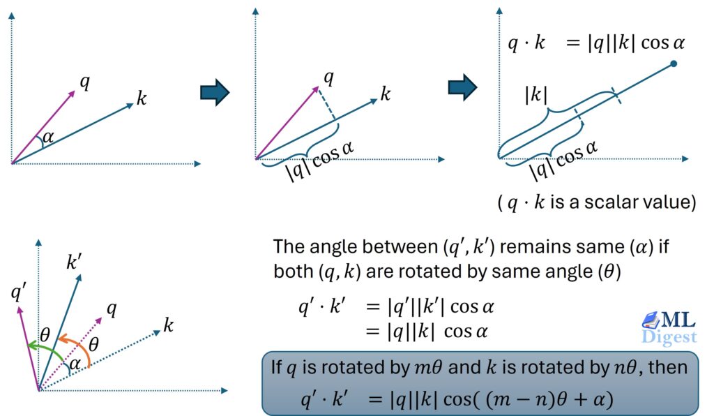
Let us start with a simple 2-dimensional vector. We have a query vector \(q\) at position \(m\) and a key vector \(k\) at position \(n\).
- We rotate \(q\) by angle \(m\theta\) to get \(q’\).
- We rotate \(k\) by angle \(n\theta\) to get \(k’\).
The dot product \(\langle q’, k’ \rangle\) which determines the attention score, is invariant to a global rotation. This means we can rotate the entire system by \(-n\theta\) without changing the result. If we do this:
- \(k’\) rotates back to the original \(k\).
- \(q’\) rotates by \(m\theta – n\theta = (m-n)\theta\).
So, the dot product \(\langle q’, k’ \rangle\) is the same as the dot product between the original query \(q\) and a key vector \(k\) that has been rotated by the relative angle \((m-n)\theta\). The calculation now only depends on the relative distance, not the absolute positions.
Thus, if we rotate both the query vector \(q\) (at position \(m\)) and the key vector \(k\) (at position \(n\)) using RoPE, their dot product becomes dependent only on their original embeddings and their relative distance (\(m-n\)). The absolute positions \(m\) and \(n\) magically disappear from the final dot product calculation.
The 2D Case
We can represent a 2D vector \((x_1, x_2)\) as a complex number \(z = x_1 + i x_2\).
To rotate this vector by an angle dependent on position \(m\), we multiply it by \(e^{im\theta}\):
$$
f(x, m) = x \cdot e^{im\theta}
$$
Using Euler’s formula (\(e^{i\theta} = \cos \theta + i \sin \theta\)), this multiplication in the complex plane corresponds to a matrix multiplication in the real plane:
$$
\begin{pmatrix} x’_1 \\ x’_2 \end{pmatrix} = \begin{pmatrix} \cos m\theta & -\sin m\theta \\ \sin m\theta & \cos m\theta \end{pmatrix} \begin{pmatrix} x_1 \\ x_2 \end{pmatrix}
$$
The “Relative” Magic
Why does this work? Let us look at the dot product (attention score) between a query at position \(m\) and a key at position \(n\). In the complex domain, the dot product corresponds to the real part of the product of one number and the conjugate of the other:
$$
\langle f(q, m), f(k, n) \rangle = \text{Re}(q e^{im\theta} \cdot \overline{k e^{in\theta}})
$$
$$
= \text{Re}(q \overline{k} e^{i(m-n)\theta})
$$
Notice the term \((m-n)\). The result depends only on the relative distance between positions \(m\) and \(n\), not on \(m\) or \(n\) individually. This is the core mathematical property that makes RoPE so powerful.
Generalizing to $d$ Dimensions
Neural networks work with high-dimensional vectors (e.g., \(d=512\) or \(d=4096\)), not just 2D. RoPE handles this by dividing the \(d\)-dimensional vector into \(d/2\) pairs. It applies a 2D rotation to each pair independently.
For a vector \(x = [x_1, x_2, x_3, x_4, \dots, x_d]\), we pair them as \((x_1, x_2), (x_3, x_4)\), etc. Each pair gets its own frequency \(\theta_i\).
The rotation matrix becomes a block-diagonal matrix:
$$
R_{\Theta, m} = \begin{pmatrix}
\cos m\theta_1 & -\sin m\theta_1 & 0 & 0 & \cdots \\
\sin m\theta_1 & \cos m\theta_1 & 0 & 0 & \cdots \\
0 & 0 & \cos m\theta_2 & -\sin m\theta_2 & \cdots \\
0 & 0 & \sin m\theta_2 & \cos m\theta_2 & \cdots \\
\vdots & \vdots & \vdots & \vdots & \ddots
\end{pmatrix}
$$
Usually, the frequencies \(\theta_i\) are defined as \(\theta_i = 10000^{-2(i-1)/d}\), similar to the original sinusoidal encoding frequencies.
A query vector \(q\) at position \(m\) is transformed into \(q_m\) by applying this rotation:
$$
q_m = R_{\Theta, m} q
$$
Similarly, a key vector \(k\) at position \(n\) is transformed into \(k_n\):
$$
k_n = R_{\Theta, n} k
$$
The attention score is then the dot product \(q_m^T k_n\). Because rotation matrices are orthogonal (\(R^T R = I\)), the dot product simplifies beautifully:
$$
q_m^T k_n = (R_m q)^T (R_n k) = q^T R_m^T R_n k = q^T R_{m-n} k
$$
This final equation is the magic of RoPE. The dot product between the query at position \(m\) and the key at position \(n\) depends only on their original embeddings (\(q\) and \(k\)) and the rotation matrix for their relative distance \(m-n\). The absolute positions are gone, leaving only the relative relationship.
Another key benefit is that the magnitude of the dot product naturally decays as the relative distance \(|m-n|\) increases, because the rotations for distant tokens are more likely to misalign them. This is a desirable property, as closer words are often more relevant to each other.
Implementation: RoPE in PyTorch
Let us translate this theory into clean, efficient Python code. We will implement a module that pre-computes the cosine and sine values (since they are fixed for each position) and applies the rotation efficiently.
import torch
import torch.nn as nn

class RotaryPositionalEmbeddings(nn.Module):
    def __init__(self, d_model: int, max_seq_len: int = 4096, base: int = 10000):
        """
        Args:
            d_model: The dimension of the embedding vector (must be even).
            max_seq_len: The maximum sequence length to pre-compute.
            base: The base for the geometric progression of frequencies.
        """
        super().__init__()
        self.d_model = d_model

        # 1. Create the frequency bands (theta_i)
        # We only need d_model / 2 frequencies because we process pairs.
        theta = 1.0 / (base ** (torch.arange(0, d_model, 2).float() / d_model))

        # 2. Create the position indices (m)
        position = torch.arange(max_seq_len).float()

        # 3. Compute the outer product m * theta
        # Shape: (max_seq_len, d_model / 2)
        freqs = torch.outer(position, theta)

        # 4. We need to apply these to both parts of the pair (x1 and x2).
        # We repeat the frequencies to match the shape of the full vector.
        # Shape: (max_seq_len, d_model)
        # Example: [theta_1, theta_2] -> [theta_1, theta_1, theta_2, theta_2]
        emb = torch.cat((freqs, freqs), dim=-1)

        # Register as a buffer so it is part of the state_dict but not a trainable parameter
        self.register_buffer("cos_cached", emb.cos())
        self.register_buffer("sin_cached", emb.sin())

    def forward(self, x):
        """
        Args:
            x: Input tensor of shape (batch_size, seq_len, n_heads, head_dim)
        Returns:
            Tensor with rotary embeddings applied.
        """
        # Slice the cached cos/sin to the current sequence length
        seq_len = x.shape[1]
        cos = self.cos_cached[:seq_len, :].unsqueeze(0).unsqueeze(2)
        sin = self.sin_cached[:seq_len, :].unsqueeze(0).unsqueeze(2)

        return self.apply_rotary_emb(x, cos, sin)

    def apply_rotary_emb(self, x, cos, sin):
        # To rotate (x1, x2), we calculate:
        # x1_new = x1 * cos - x2 * sin
        # x2_new = x1 * sin + x2 * cos

        # Helper to get [-x2, x1, -x4, x3, ...]
        def rotate_half(x):
            x1, x2 = x[..., :x.shape[-1]//2], x[..., x.shape[-1]//2:]
            return torch.cat((-x2, x1), dim=-1)

        return (x * cos) + (rotate_half(x) * sin)

# Example Usage
if __name__ == "__main__":
    batch_size = 2
    seq_len = 10
    n_heads = 4
    head_dim = 64 # d_model per head

    # Initialize RoPE
    rope = RotaryPositionalEmbeddings(d_model=head_dim)

    # Dummy Query and Key vectors
    q = torch.randn(batch_size, seq_len, n_heads, head_dim)
    k = torch.randn(batch_size, seq_len, n_heads, head_dim)

    # Apply rotation
    q_rotated = rope(q)
    k_rotated = rope(k)

    print(f"Original shape: {q.shape}")
    print(f"Rotated shape:  {q_rotated.shape}")
# The attention score calculation (q @ k.T) will now contain relative position info!Key Advantages of RoPE
RoPE’s design offers several significant advantages over traditional positional embedding methods, making it a preferred choice for modern LLMs.
Implicit Relative Encoding
The core strength of RoPE is its ability to encode relative positional information implicitly. As shown in the mathematical derivation, the dot product between a query at position m and a key at position n depends only on their relative distance (m-n).
Why this helps with coherence in long sequences:
Language is built on relative relationships. The meaning of a word is often determined by its neighbors, not its absolute position in a document. By focusing on relative distance, RoPE allows the attention mechanism to learn patterns that are position-agnostic. For example, it can learn the relationship between an adjective and the noun that follows it, regardless of whether this pair appears at the beginning or end of a sentence. This leads to more robust and coherent understanding, especially in long sequences where absolute positions become less meaningful.
Extrapolation Beyond Training Context Lengths
RoPE demonstrates remarkable extrapolation capabilities, allowing models to handle sequences longer than those seen during training.
Scaling behaviors:
Because RoPE is based on continuous rotations, it does not have a hard “edge” or a fixed maximum length like absolute embeddings. The model learns to interpret the rotational angles. While performance can degrade over very long distances due to periodic effects, the decay is gradual.
Why models like LLaMA can extend context with minimal retraining:
This property is exploited by models like LLaMA to extend their context windows. By using techniques like NTK-aware scaling to adjust the rotation frequencies (\(\theta\) values) at inference time, the model can effectively “zoom out,” accommodating longer sequences without having been explicitly trained on them. This allows for extending context with only minimal fine-tuning, a significant advantage over methods that would require complete retraining.
Smoothness and Continuity
The use of sinusoidal functions for rotation means that the positional representation is smooth and continuous. The change from one position to the next is a small, incremental rotation rather than a jump to a completely different embedding vector.
Benefits for attention stability:
This continuity helps stabilize the attention mechanism. The model learns in a more predictable space, where small changes in position lead to small changes in the query/key representations. This can lead to smoother training and more stable attention scores, as the model is not forced to learn abrupt changes between adjacent positions.
Parameter Efficiency and Simplicity
RoPE is highly efficient and simple to implement.
No trainable parameters:
Unlike some relative position embedding schemes, RoPE introduces no new trainable parameters. The positional information is generated by a fixed function, which reduces model size and eliminates the need to learn positional representations from data.
Easy drop-in replacement for sinusoidal embedding:
From an implementation perspective, RoPE is a clean modification. It reuses the same frequency-based formulation as the original Transformer’s sinusoidal embeddings but applies it through multiplication (rotation) instead of addition. This makes it a relatively straightforward “drop-in” enhancement for many Transformer architectures.
Variants and Extensions of RoPE
The elegance and effectiveness of RoPE have inspired a family of variants and extensions. Most of these aim to improve its ability to handle extremely long contexts or to fine-tune its behavior for specific tasks.
- Scaling Methods for Long Contexts (PI, NTK, YaRN):
A key challenge is maintaining performance when extrapolating to sequences much longer than the model’s training length. Naive extrapolation can cause issues as the rotational angles become very large.- Position Interpolation (PI): A simple approach that scales down the position indices to fit within the original trained context size (e.g., treating a sequence of length 8192 as if it were 2048). While easy to implement, it can degrade performance by losing high-frequency details.
- NTK-Aware Scaling: This method provides a more principled way to adapt RoPE to longer contexts by adjusting the base of the frequency calculation. It effectively increases the “wavelength” of the positional encodings, allowing the model to interpolate more smoothly over longer distances.
- YaRN (Yet another RoPE extensioN): A state-of-the-art technique that builds on NTK-aware scaling. YaRN intelligently scales the RoPE frequencies while also scaling the query and key tensors themselves. This helps to re-introduce the high-frequency information that can be lost with other scaling methods, achieving a better balance between long-context stability and preserving fine-grained details.
- LongRoPE/LongRoPE2:
These are specialized methods designed for scaling context windows to extreme lengths (e.g., up to 2 million tokens). They often combine sophisticated scaling techniques with modifications to the attention mechanism itself to manage the computational and memory challenges of such vast contexts. - xPos: RoPE with Exponential Decay:
While RoPE’s dot product naturally decays with distance,xPosmakes this decay explicit and learnable. It introduces an exponential decay factor that is applied to the rotated embeddings based on their relative distance. This gives the model more direct, trainable control over how attention scores fall off with distance, which can be beneficial for tasks requiring more nuanced attention patterns. - Directional RoPE (DRoPE):
Standard RoPE is symmetric, meaning the encoding for a relative distance of+kis the transpose of the encoding for-k. DRoPE breaks this symmetry by introducing a mechanism that allows the model to distinguish more effectively between the forward and backward directions in a sequence. This can be particularly useful for tasks where causality and temporal order are critical. - Linearized RoPE and Efficiency Variants:
To overcome the quadratic complexity of the standard attention mechanism, some research has explored ways to linearize attention when used with RoPE. These methods aim to express the RoPE-based attention mechanism as a linear recurrence, which can reduce the computational complexity fromO(N^2)toO(N). This is especially valuable for achieving very fast inference in autoregressive generation.
Practical Tips and Best Practices
When integrating RoPE into your models, consider the following insights to maximize performance and stability.
1. Where to Apply It
RoPE is applied at every layer, specifically to the Query (\(q\)) and Key (\(k\)) vectors before the attention mechanism computes the dot product. Do not apply it to the Value (\(v\)) vectors. This ensures that the attention scores (the “where to look” signal) are position-aware, while the content retrieved (the “what to retrieve” signal) remains pure.
2. Extrapolation Capabilities
One of the strongest arguments for RoPE is its ability to handle sequence lengths longer than what it was trained on (length extrapolation). Because it relies on rotation (which is periodic) rather than absolute indices, models using RoPE tend to degrade more gracefully on long sequences compared to learned absolute embeddings.
- Tip: If you need to extend the context window of a pre-trained LLaMA model (which uses RoPE), look into “Linear Scaling” or “NTK-Aware Scaling” of the RoPE frequencies. These techniques adjust the rotation speed to map longer sequences into the trained rotation range.
3. Computational Efficiency
RoPE is computationally cheap. It involves element-wise multiplications and additions, which are negligible compared to the matrix multiplications in the attention layers.
- Optimization: In the implementation above, we cache the
cosandsintables. Ensure you slice these tables correctly during inference to match the current sequence length, avoiding re-computation at every step.
4. Compatibility with Linear Attention
Standard RoPE relies on the specific interaction in the softmax attention mechanism (\(\text{Re}(q \overline{k} e^{i(m-n)\theta})\)). If you are experimenting with “Linear Attention” or other kernel-based attention variants that do not compute the full \(QK^T\) matrix, RoPE might not be directly applicable or may require mathematical adjustments.
Conclusion
Rotary Positional Embeddings represent a shift from viewing position as a static label to viewing it as a geometric relationship. By treating tokens as vectors rotating in high-dimensional space, we allow neural networks to understand that “King” is to “Queen” not just by their semantic meaning, but by their relative placement in the text.
It is a mathematically elegant solution that has become the standard for modern LLMs. Understanding RoPE is understanding the engine under the hood of today’s most capable AI systems.

Happy is a seasoned ML professional with over 15 years of experience. His expertise spans various domains, including Computer Vision, Natural Language Processing (NLP), and Time Series analysis. He holds a PhD in Machine Learning from IIT Kharagpur and has furthered his research with postdoctoral experience at INRIA-Sophia Antipolis, France. Happy has a proven track record of delivering impactful ML solutions to clients.
Subscribe to our newsletter!