For Large Language Models (LLMs), inference speed and efficiency are paramount. One of the most critical optimizations for speeding up text generation is KV-Caching (Key-Value Caching).
If you have ever wondered why generating text with GPT-4 or Llama 2 gets slower as the conversation gets longer, or how these models manage to “remember” the context without re-processing the entire history every single time, the answer lies in how they handle the Keys (K) and Values (V) of the attention mechanism.
Intuitively, KV caching converts the habit of “re-reading the entire book before writing each new sentence” into “consulting detailed notes and appending only the newest sentence.”
The Intuition: The “Re-reading” Analogy
Imagine you are writing a novel. You are currently on page 100. To write the first sentence of page 101, you need to recall the plot points, character arcs, and setting details from the first 100 pages.
Without KV-Caching (Naive Approach):
Every time you want to write a new word, you re-read the entire book from page 1 to page 100 to refresh your memory.
- To write word 1 on page 101: Read pages 1-100.
- To write word 2 on page 101: Read pages 1-100 plus word 1.
- To write word 3 on page 101: Read pages 1-100 plus words 1 and 2.
This is obviously inefficient. As the book gets longer, writing becomes excruciatingly slow.
With KV-Caching:
You read pages 1-100 once and take detailed notes (the Cache).
- To write word 1 on page 101: Look at your notes, write the word, and update your notes with this new word.
- To write word 2: Look at your updated notes, write the word, and update the notes again.
You never re-read the old pages. You simply append the new information to your running summary. In LLM terms, this “running summary” consists of the Key and Value matrices computed for previous tokens.
The Problem: Autoregressive Generation Bottlenecks
LLMs generate text autoregressively, meaning they produce one token at a time, and each new token depends on all previous tokens.
In the standard Transformer attention mechanism, calculating the output for the current token requires the model to “attend” to all previous tokens. To avoid ambiguity, define the per-head dimension as \(d_{h}\) (i.e., \(d_{h} = d_{\mathrm{model}}/h\) where \(h\) is the number of heads).
Mathematically, for a sequence of length \(t\), the attention layer computes Query (\(Q\)), Key (\(K\)), and Value (\(V\)) matrices from the input embeddings and applies scaled dot-product attention:
$$
\mathrm{Attention}(Q, K, V) = \mathrm{softmax}\left(\frac{QK^{T}}{\sqrt{d_{h}}}\right)V.
$$
If we generate the sequence “The cat sat”, the steps look like this without caching:
- Input “The”: Compute \(Q_1, K_1, V_1\). Output “cat”.
- Input “The cat”: Compute \(Q_1, K_1, V_1\) AND \(Q_2, K_2, V_2\). Output “sat”.
- Input “The cat sat”: Compute \(Q_1, K_1, V_1\) AND \(Q_2, K_2, V_2\) AND \(Q_3, K_3, V_3\). Output “on”.
Notice the redundancy? We re-computed \(K_1, V_1\) in step 2 and step 3, even though they never change!
Without caching, at generation time every new step re-projects previous token embeddings into K and V vectors, even though those projections are identical to the ones computed for earlier steps. KV caching prevents that redundancy by storing K and V tensors for earlier tokens and reusing them.
The Solution: Caching Keys and Values
KV-Caching eliminates this redundant computation. Instead of re-calculating the Key and Value vectors for past tokens, we store them in GPU memory (VRAM) and retrieve them when needed.
Mathematical Formulation
Let’s look at the attention calculation for the token at time step \(t\) (the current token we are processing).
- Compute Current Vectors: We only process the newest token \(x_t\) through the projection layers to get its query, key, and value vectors:
$$
q_t = x_t W_Q, \quad k_t = x_t W_K, \quad v_t = x_t W_V
$$ - Retrieve and Append: We fetch the cached keys and values from previous steps (\(K_{past}, V_{past}\)) and concatenate the new \(k_t\) and \(v_t\):
$$
K_{current} = [K_{past} ; k_t]
$$
$$
V_{current} = [V_{past} ; v_t]
$$ - Attend: We compute attention using the current query \(q_t\) against the entire history \(K_{current}\) and \(V_{current}\):
$$
\mathrm{Attention}_{t} = \mathrm{softmax}\left(\frac{q_{t}K_{current}^{T}}{\sqrt{d_{h}}}\right)V_{current}.
$$ - Update Cache: The new \(K_{current}\) and \(V_{current}\) become the cache for the next step.
Note: We do not cache the Query (\(Q\)) vectors. Why? Because the query is only used to find relationships from the current token to the past tokens. Once the current token is processed, its query vector is no longer needed for future tokens.

Important nuance: KV caching avoids recomputing previous projections, but the attention score computation for the current query still scales with the length of the cached sequence. Therefore, while caching reduces repeated projection overhead substantially, the attention score multiplication remains linear in the sequence length per step; the total work across a full sequence still exhibits quadratic growth in sequence length, but with a much smaller constant factor.
Python Implementation
Here is a simplified implementation of a Self-Attention layer with KV-Caching support.
import torch
import torch.nn as nn
import torch.nn.functional as F

class CausalSelfAttention(nn.Module):
    """Causal self-attention with KV caching.

    Args:
        d_model: model dimension.
        n_head: number of attention heads.
    """

    def __init__(self, d_model, n_head):
        super().__init__()
        self.d_h = d_model // n_head
        self.n_head = n_head
        self.d_model = d_model

        # Projections
        self.W_q = nn.Linear(d_model, d_model, bias=False)
        self.W_k = nn.Linear(d_model, d_model, bias=False)
        self.W_v = nn.Linear(d_model, d_model, bias=False)
        self.W_o = nn.Linear(d_model, d_model, bias=False)

    def forward(self, x, past_kv=None):
        """
        x: Input tensor of shape (batch_size (B), seq_len, d_model)
           During generation, seq_len is usually 1 (the current token).
        past_kv: Tuple of (K_cache, V_cache) from previous step.
        """
        B, seq_len, _ = x.shape

        # 1. Compute Q, K, V for the *current* input x
        q = self.W_q(x).view(B, seq_len, self.n_head, self.d_h).transpose(1, 2)
        k = self.W_k(x).view(B, seq_len, self.n_head, self.d_h).transpose(1, 2)
        v = self.W_v(x).view(B, seq_len, self.n_head, self.d_h).transpose(1, 2)

        # 2. If we have a cache, concatenate with past keys/values
        if past_kv is not None:
            past_k, past_v = past_kv
            k = torch.cat([past_k, k], dim=2) # Concatenate along sequence dimension
            v = torch.cat([past_v, v], dim=2)

        # Update the cache for the next step
        current_kv = (k.detach(), v.detach())  # detach to avoid accidental grad retention

        # 3. Compute Attention
        # q shape: (batch, n_head, 1, d_h)
        # k shape: (batch, n_head, total_seq_len, d_h)
        scores = (q @ k.transpose(-2, -1)) / (self.d_h ** 0.5)

        # Apply causal mask if needed (omitted for brevity in single-token step)
        attn_weights = F.softmax(scores, dim=-1)

        output = attn_weights @ v # (batch, n_head, 1, d_h)

        # Reassemble heads
        output = output.transpose(1, 2).contiguous().view(B, seq_len, self.d_model)
        return self.W_o(output), current_kv

# --- Example Usage ---

# Hyperparameters
d_model = 512
n_head = 8
model = CausalSelfAttention(d_model, n_head)

# Dummy input (batch=1, seq_len=1) representing the current token
x_t = torch.randn(1, 1, d_model)
past_kv = None

# Generation Loop
for i in range(5):
    output, past_kv = model(x_t, past_kv=past_kv)
    print(f"Step {i}: Cache size (seq_len) = {past_kv[0].shape[2]}")

    # In a real model, we would sample the next token here.
    # For this example, we just use random input for the next step.
x_t = torch.randn(1, 1, d_model)Memory and Computation Trade-offs
While KV-Caching drastically improves computation speed (FLOPs), it introduces a new bottleneck: Memory Capacity.
The Memory Wall
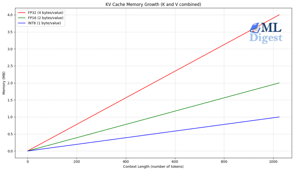
The KV cache grows linearly with the sequence length. For very long sequences (e.g., 100k tokens), the cache can become massive, potentially exceeding the GPU’s VRAM.
Size Calculation:
For a model with:
- \(L\) layers
- \(d_{model}\) hidden dimension
- \(B\) batch size
- \(t\) sequence length
- Precision \(P\) (e.g., 2 bytes for float16)
The size of the KV cache is roughly:
$$
\text{Size} \approx 2 \times L \times B \times t \times d_{model} \times P
$$
(The factor of 2 is for storing both K and V).
For a 7B parameter model (like Llama 2) with a batch size of 1 and sequence length of 4096, the cache can take up hundreds of megabytes. With larger batches, it quickly reaches gigabytes.
Compute vs. Memory Bandwidth
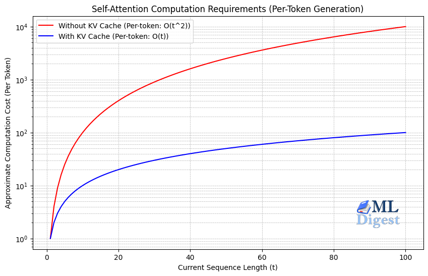
- Without Cache: Compute-bound. The GPU spends most of its time doing matrix multiplications. The attention computation cost for GENERATING A SINGLE TOKEN at current sequence length \(t\) is quadratic \(O(t^2)\), because the entire sequence up to that point needs to be recomputed. Memory access is relatively small compared to compute.
- With Cache: Memory-bandwidth bound. The GPU spends most of its time moving the large KV cache from VRAM to the compute cores. The computation cost for GENERATING A SINGLE TOKEN at current sequence length \(t\) is linear, \(O(t)\), because only the current token needs to attend to the t tokens already in the cache. But the memory access pattern becomes the bottleneck.
Practical Tips and Best Practices
- Pre-allocation:
In optimized inference engines (like vLLM or TGI), memory for the KV cache is often pre-allocated in blocks to avoid fragmentation and overhead during generation. - PagedAttention:
Inspired by virtual memory in operating systems, PagedAttention (used in vLLM) splits the KV cache into non-contiguous blocks. This allows the system to handle memory much more flexibly, reducing waste and allowing for larger batch sizes. - Quantization:
To save memory, you can store the KV cache in lower precision (e.g., 8-bit or 4-bit integers) instead of float16. This is called KV Cache Quantization. It slightly reduces generation quality but significantly reduces memory usage, allowing for longer context windows. - Multi-Query Attention (MQA) & Grouped-Query Attention (GQA):
Modern architectures like Llama 2 and Falcon use GQA or MQA. These techniques share Key and Value heads across multiple Query heads. This drastically reduces the size of the KV cache (\(d_{model}\) in the formula above becomes much smaller), enabling faster inference and longer contexts.- Standard: 1 KV head per Query head.
- MQA: 1 KV head for all Query heads.
- GQA: 1 KV head for a group of Query heads.
Summary
- KV-Caching is essential for efficient autoregressive text generation.
- It works by storing the Key and Value vectors of past tokens so they don’t need to be re-computed.
- It changes the complexity of the attention step from quadratic \(O(t^2)\) (re-computing everything) to linear \(O(t)\) (computing only the new token) with respect to the total work done over the sequence.
- The principal trade-off is memory (VRAM usage): the cache grows with layers, heads, batch size, and sequence length, which shifts the bottleneck to memory capacity and bandwidth.
- Techniques like GQA, PagedAttention, head-sharing, and Quantization are critical for managing this memory footprint in production.
Resources

Happy is a seasoned ML professional with over 15 years of experience. His expertise spans various domains, including Computer Vision, Natural Language Processing (NLP), and Time Series analysis. He holds a PhD in Machine Learning from IIT Kharagpur and has furthered his research with postdoctoral experience at INRIA-Sophia Antipolis, France. Happy has a proven track record of delivering impactful ML solutions to clients.
Subscribe to our newsletter!