Deep Learning Optimization: The Role of Layer Normalization

Layer normalization has emerged as a pivotal technique in the optimization of deep learning models, particularly when it comes to training stability and performance enhancement. This article delves into the mechanics of layer normalization, its mathematical foundation, and its applications across various types of neural networks. We will also compare it with other normalization techniques, specifically batch normalization and instance normalization, and discuss its advantages and limitations.

Layer normalization (LayerNorm) is a technique used to normalize the inputs of each layer in a neural network.

Importance of Normalization

Normalization techniques seek to stabilize and accelerate the training of neural networks. Training deep learning models involves gradient descent methods sensitive to the distribution of input activations. Several problems prominently arise:

• Internal Covariate Shift: During training, the distribution of the inputs to each layer changes as the parameters of the previous layers are updated. This can lead to poor convergence properties and require more careful tuning of hyperparameters.
• Exploding and Vanishing Gradients: In very deep networks, gradients can either become very large (exploding) or very small (vanishing), making it difficult for the neural network to learn effectively.

Normalization methods aim to address these issues by standardizing the inputs to a layer, ensuring that the network learns more efficiently and effectively.

What is Layer Normalization?

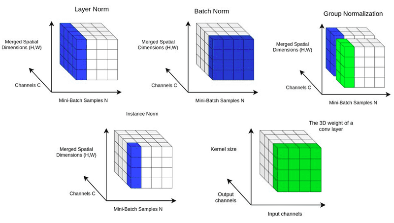
Introduced by Ba et al. (2016), layer normalization targets the normalization of the output of a layer for an individual sample, unlike batch normalization (BatchNorm) which normalizes over the entire mini-batch. It computes the mean and variance for each feature dimension per example rather than per batch, which makes it suited for RNNs and transformers where batch sizes can vary or be small.

Mathematical Formulation

Given an input vector \( a \) with \( H \) dimensions (features), where \( H \) refers to the number of hidden units in a layer, the layer normalization process can be described in a series of steps:

1. Compute the Mean:
   \[
   \mu = \frac{1}{H} \sum_{i=1}^{H} a_i
   \]
2. Compute the Variance:
   \[
   \sigma^2 = \frac{1}{H} \sum_{i=1}^{H} (a_i – \mu)^2
   \]
3. Normalize the Input:
   \[
   \hat{a_i} = \frac{a_i – \mu}{\sqrt{\sigma^2 + \epsilon}}
   \]
   Where \( \epsilon \) is a small constant added to prevent division by zero.
4. Scale and Shift:
   After normalization, the output is scaled and shifted using learnable parameters \( \gamma \) and \( \beta \):
   \[
   y_i = \gamma \hat{a_i} + \beta
   \]
   where \( \gamma \) and \( \beta \) are parameters that allow the model to undo the normalization if necessary.

Computational Complexity

The computational cost associated with layer normalization is relatively low. Performing mean and variance calculations followed by normalization for each instance is efficient, especially in scenarios with batch sizes of 1—common in RNNs. The operations are performed in \( O(NH) \) for \( N \) instances and \( H \) features, which is feasible even for larger models.

Implementation

Layer normalization can be implemented easily in popular deep learning frameworks such as TensorFlow and PyTorch. Here’s a simplified example in PyTorch:

import torch
import torch.nn as nn

class LayerNormExample(nn.Module):
    def __init__(self, num_features):
        super(LayerNormExample, self).__init__()
        self.layer_norm = nn.LayerNorm(num_features)

    def forward(self, x):
        return self.layer_norm(x)

This implementation uses PyTorch’s built-in LayerNorm, which automatically handles the computations related to mean, variance, and scaling.

Comparison with Other Normalization Techniques

• Batch Normalization: While layer normalization operates on the per-example basis, batch normalization computes statistics across a mini-batch, making it computationally efficient for large batch sizes. However, it can be less effective when batch sizes are small or vary significantly, as it may not provide a robust estimate of the mean and variance.
• Instance Normalization: Frequently used in style transfer applications, instance normalization normalizes each feature channel independently for each training instance. While beneficial for controlling style representations, instance normalization may not always capture the correlations across features, which layer normalization can.
• Group Normalization: Group normalization strikes a balance between instance and batch normalization by dividing channels into groups. While effective, it may still introduce some level of batch dependency, which is absent in layer normalization.

Advantages of Layer Normalization

• Independence from Batch Size: Due to its per-example treatment, layer normalization is robust when facing small batch sizes, making it ideal for tasks where such conditions are prevalent, like RNNs, transformers, and Reinforcement Learning.
• Invariance to Batch Order: Because layer normalization normalizes individual examples, the outcomes are not influenced by the ordering of input samples within a batch, leading to more stable training dynamics.
• Improved Generalization: Layer normalization has been shown to improve generalization performance, particularly in high-dimensional spaces and complex architectures, by stabilizing the learning process.
• Flexibility in Model Design: The incorporation of learnable parameters enables layer normalization to be adaptable to different types of feature distributions, retaining the representational power and expressiveness of the model.

Limitations

• Computational Overhead: The per-sample normalization incurs additional computational cost, particularly for large feature dimensions when compared with batch normalization.
• Loss of Information in Large Batches: As normalizing across the entire dimension of features for individual samples can potentially mask behavior that might emerge when observing a broader context in a batch.
• Limited Efficacy in Some Applications: Certain tasks, especially those involving spatial hierarchies or local patterns, may benefit more from batch normalization or other normalization techniques that can capture broader contextual dependencies.
• Sensitivity to Initialization: Layer normalization can be sensitive to the initialization of parameters, requiring careful tuning to ensure optimal performance.

Applications of Layer Normalization

• Natural Language Processing: Layer normalization has been instrumental in the design of transformer architectures used in models like BERT and GPT, allowing effective training dynamics over long sequences.
• Generative Models: It has been utilized in various generative models, consciously attempting to regulate learning representations while retaining the ability for expressive modeling.
• Recurrent Neural Networks: Many RNN architectures benefit from layer normalization due to its individual normalization approach, which helps in stabilizing updates across time steps effectively.
• Robustness in Unstructured Data: In tasks such as image captioning, video processing, and unsupervised learning, where batch sizes can vary and may not yield independent distribution assumptions, layer normalization has shown promise.